The COPILOT Raw Illumina Genotyping QC Protocol
Hamel Patel, Hamel Patel, Sang-Hyuck Lee, Sang-Hyuck Lee, Gerome Breen, Gerome Breen, Stephen Menzel, Stephen Menzel, Oyesola Ojewunmi, Oyesola Ojewunmi, Richard J.B. Dobson, Richard J.B. Dobson
Abstract
The Illumina genotyping microarrays generate data in image format, which is processed by the platform-specific software GenomeStudio, followed by an array of complex bioinformatics analyses that rely on various software, different programming languages, and numerous dependencies to be installed and configured correctly. The entire process can be time-consuming, can lead to reproducibility errors, and can be a daunting task for bioinformaticians. To address this, we introduce the COPILOT protocol, which has been successfully used to transform raw Illumina genotype intensity data into high-quality analysis-ready data on tens of thousands of human patient samples that have been genotyped on a variety of Illumina genotyping arrays. This includes processing both mainstream and custom content genotyping chips with over 4 million markers per sample.
The COPILOT QC protocol consists of two distinct tandem procedures to process raw Illumina genotyping data. The first protocol is an up-to-date process to systematically QC raw Illumina microarray genotyping data using the Illumina-specific GenomeStudio software. The second protocol takes the output from the first protocol and further processes the data through the COPILOT (C ontainerised wO rkflow for P rocessing IL lumina genO typing daT a) containerized QC pipeline, to automate an array of complex bioinformatics analyses to improve data quality through a secondary clustering algorithm and to automatically identify typical Genome-Wide Association Study (GWAS) data issues, including gender discrepancies, heterozygosity outliers, related individuals, and population outliers, through ancestry estimation. The data is returned to the user in analysis-ready PLINK binary format and is accompanied by a comprehensive and interactive HTML summary report file which quickly helps the user understand the data and guides the user for further data analyses. The COPILOT protocol and containerized pipeline are also available at https://khp-informatics.github.io/COPILOT/index.html. © 2022 The Authors. Current Protocols published by Wiley Periodicals LLC.
Basic Protocol 1 : Processing raw Illumina genotyping data using GenomeStudio
Basic Protocol 2 : COPILOT: A containerised workflow for processing Illumina genotyping data
INTRODUCTION
A genome-wide association study (GWAS) is an approach to identify genetic variants associated with a particular disease or phenotypic trait. Microarray-based GWAS remains a common approach for identifying these genetic associations across the whole genome. The Illumina genotyping arrays accomplish this by using pre-defined oligonucleotide probes designed to hybridize specific regions of genomic DNA, followed by extension using chemically labeled nucleotides. The probe extension binds either red or green fluorescent agents, which can be interpreted by the Illumina-specific software GenomeStudio. This software determines the identity of alleles by automated clustering of samples based on the similarity of fluorescent intensity. However, the default clustering algorithm can fail to identity valid clusters and can also assign the wrong genotype to samples due to abnormal intensity patterns. This can be addressed by manually reviewing and recalling SNPs to increase the reliability, confidence, and overall quality of the data (SNP/sample call rates), making this an extremely crucial quality control (QC) procedure prior to further QC using PLINK or genetic interpretation.
Through processing tens of thousands of human patient samples from various tissue sources and on a variety of Illumina genotyping arrays, including both mainstream and custom content genotyping chips with over 4 million markers per sample, we have accumulated extensive hands-on experience in processing raw Illumina genotype data for numerous genetic investigations (Coleman et al., 2016; Fabbri et al., 2018; Gardner et al., 2018; Harrison et al., 2017; Santoro et al., 2018; Traylor et al., 2017; Vassos et al., 2017; Voyle et al., 2017). We translate this knowledge and experience in this article into a detailed easy-to-follow step-by-step procedure, allowing users to effortlessly transform raw Illumina genotype intensity data to high-quality analysis-ready data.
Basic Protocol 1 walks a user through the initial QC processing of raw Illumina genotype intensity data using the Illumina-specific software called GenomeStudio. The protocol includes the initial setup of the software, loading of data, QC of internal standards, QC of genotype data using up-to-date criteria to identify and address problematic samples and SNPs, and exporting the processed data. Basic Protocol 2 describes how to use the COPILOT container to automate an array of complex bioinformatics analyses to further process and improve data quality, generate PLINK format analysis-ready data, and create the interactive HTML summary report.
STRATEGIC PLANNING
If the project consists of multiple batches that are genotypes at different time points, then it would be advisable to duplicate a few samples across batches to identify and address discrepancies in genotyping of the same sample across batches. When processing different batches, the clustering positions from a processed batch can be used to cluster the next batch. This will significantly speed up the QC process and will be further explained in Basic Protocol 1.
In addition, users will require a minimum of 100 samples to reliably cluster the data in GenomeStudio, or a minimum of 100 female and 100 male samples if investigating the sex chromosomes. If sample numbers are low for a given project, then samples from another project genotyped in the same laboratory and using the same genotyping array (including version) can be merged with the data of interest to increase sample numbers to allow for reliable clustering of the intensity data in GenomeStudio.
Basic Protocol 1: PROCESSING RAW ILLUMINA GENOTYPING DATA USING GenomeStudio
This protocol provides the user with complete instructions to load and thoroughly QC raw Illumina genotyping data using the Illumina GenomeStudio software. Genotype arrays contain several thousand or even millions of genetic markers on each array, which makes it impractical to visually verify every single marker. Therefore, different intensity-related criteria are used to identify genetic markers that deviate from their expected pattern and should be manually reviewed.
Necessary Resources
Hardware
- As recommended by Illumina, the following hardware recommendations are required to run GenomeStudio software:
- CPU Speed–2.0 GHz or greater
- Processor–64-bit, with 2 or more cores
- Memory–8 GB or more
- Hard Drive–100 GB or larger
- Video Display–1280 × 1024
- Operating System–Windows 7 or higher
- Specific OS Requirements–Microsoft .NET Framework 3.5
- Network Connection–1 GbE or faster
Software
- GenomeStudio genotyping (current version at writing this article is GenomeStudio v2.0.5):
Files
The input files for GenomeStudio are:
- Illumina iDat files (.dat)–These are the raw intensity files generated by the Illumina microarrays
- Illumina genotyping array manifest (.bpm)–This contains information on the target region
- Illumina sample sheet (.csv)–This contains information on the sample and is usually provided by the genotyping laboratory. Additional phenotypic information can be added to this file to aid in the QC process. The sample sheet file contains the following columns:
- 1.Sample ID
- 2.SentrixBarcode (chip barcode on which the sample has been genotyped)
- 3.SentrixPosition (position on the chip of where the sample has been genotyped)
- 4.Sample_Plate (plate ID)
- 5.Sample_Well (well position of the sample)
- 6.Sample_Group (optional: Tissue source, i.e., saliva, buccal, blood, etc…)
- 7.Gender (optional: F, M, Female or Male, with the first letter always in uppercase. Any other nomenclature will be imported as “Unknown”. Without gender information the sex chromosomes cannot be reliably processed.)
- 8.Sample_Name (optional: alias name)
- 9.Replicate (optional: specify the “Sample_Name” of any replicated samples)
- 10.Parent 1 (optional: Father's “Sample_Name” if genotyped–can be used to identify parent-child or parent-parent-child SNP discrepancies)
- 11.Parent 2 (optional: Mother's “Sample_Name” if genotyped–parent-child or parent-parent-child SNP discrepancies)
- 12.Path (Full path to data directory containing the IDAT file for the sample)
1.Configuring GenomeStudio.
GenomeStudio uses the GenCall algorithm to cluster the raw intensity data and assign genotype calls. The software has default parameters and setting which can be adjusted to speed up the internal calculations.
-
From the main window, select “Tools” > “Options” > “Project”:Check the “Exclude Female Y-SNPs from SNP Statistics” box.Ensure the “No-call Threshold” is set to 0.15.Click “Use for all New Projects”.
-
From the main window, select “Tools” > “Options” > “Module” > “Genotyping”: Check the “Use memory-based storage” box. This will massively speed up the clustering process; however, sufficient memory is required for this option. We have successfully used this option with a 32 GB RAM machine, clustering thousands of samples.
GenomeStudio will often reset these settings to default. Users are strongly advised to check these settings every time a project is created/opened.
2.Creating a new genotyping project.
-
From the main window, select “File” > “New Project” > “Genotyping” and follow the GenomeStudio Project Wizard.Under “Projects Repository”, navigate and select the folder where you want to create and store the GenomeStudio project.Under “Project Name”, create a project name, e.g., we suggest[PROJECT_NAME]_[DATE]_01.bscand click “Next”. The “_01” file will be the raw data without QC. We will save any modifications to this data as a separate file later in this protocol, which will have the same project name except it will end in “_02”, to represent a processed project.Select “use sample sheet to load sample intensities” and click “Next”.Specify sample sheet,.idatfile location, and manifest location, and click “Next”.Here we have an option to “import cluster positions from a cluster file” to cluster the data. From experience, we have discovered that using the default Illumina cluster file, or a cluster file generated from a different laboratory from which the data was generated, can lead to poor clustering. This is generally due to laboratory-specific variation leading to intensity data variations which lead to cluster drifts. We recommend not using a cluster file, but clustering the data using the data itself. Note, the clustering algorithm requires a minimum of 100 samples to work effectively. Once a Genotype project has undergone QC, the cluster positions can be exported and re-used to cluster new data genotyped on the same genotype chip. To use an existing cluster file, check the “Import cluster positions form a cluster file” box and specify the cluster file (.egt) location. Otherwise, check “Cluster SNP's”. Generating a cluster file after QC is further detailed later in this protocol.Check “Calculate Sample and SNP Statistics” and “Pre-calculate” boxes.Ensure Gen Call Threshold is set at 0.15 and click “Finish” to create the project. Depending on the computing power and number of samples/SNPs, this process may take several minutes to several hours to cluster the data and calculate the statistics.
-
Once the project has been created, check that the sample numbers in GenomeStudio match those in the sample sheet. If there are any errors in the sample sheet, a sample is not present at the location specified in the sample sheet, or the.idatfiles are corrupt for a given sample, then GenomeStudio will not upload the sample in question, and may not prompt an error. Therefore, it is vital to check that sample numbers in GenomeStudio correspond to those specified in the sample sheet.
3.Overview of GenomeStudio windows.
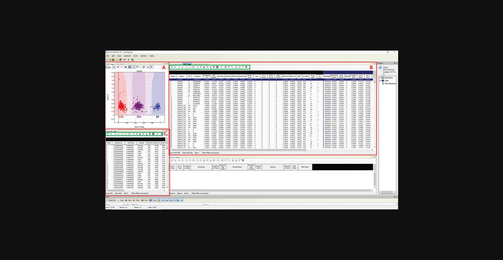
An overview of the software window is shown in Figure 1.The three main panes that will be used are (A) “SNP Graph”, which displays the intensity (green and red) of samples for a given SNP that is selected in the “SNP Table”. Samples are colored according to their genotype, where red represents AA homozygote genotype, purple represents AB heterozygote genotype, blue represents BB homozygote genotype, and black represents uncalled. The number of samples called within each cluster is displayed below the cluster. (B) “SNP Table” displays the SNP information, which includes clustering statistics, and (C) “Sample Table” displays sample information. The green boxes within the “SNP Table” and “Sample Table” panes contain options that will be used during the QC process, such as sorting of tables and filtering of rows. The remaining panes are the “Project”, “Errors Table”, and ”Log”, and should be inspected for any errors; as they are not used thereafter, they can be closed to make the remaining panes bigger and easier to view.
4.Validating internal genotyping controls.
All Illumina genotyping arrays are equipped with internal probes to verify the accuracy and reproducibility of the assay. These internal controls should be checked before the individual sample or SNP QC to verify the reliability of the data. The internal controls do not have specific threshold criteria due to differing intensities across genotype assays. Therefore, the internal controls are based on relative intensities and should be checked according to the Illumina “evaluation of Infinium genotyping assay control training guide”, which is available on the Illumina website https://static.yanyin.tech/literature/current_protocol/10.1002/cpz1.373/original_pdf/cpz1.373.pdf (Illumina, 2012).
To view the internal controls, from the main window, click on “Analysis” > “View Controls dashboard”.
5.Manually editing clusters.
During this protocol, SNPs may need to be manually edited to correctly cluster samples. To manually edit a cluster:
-
From the “SNP Graph” pane, press and hold the Shift key, and move the cursor to the center of a cluster. Once you are at the middle of the cluster, over the “+”, the cursor head will turn from an arrow to a directional “+” symbol.
-
Once the cursor head has turned into a “+”, left click and hold, and drag the cluster to the desired location
Alternatively, users can select samples they would like to exclude/include from a cluster, and GenomeStudio will attempt to exclude/include these samples.
- c.From the “SNP Graph” window, draw a box (left click and drag the cursor) around the sample(s) you want to include/exclude from a cluster.
- d.Right-click on the highlighted sample(s) and choose from the following self-explanatory options:
- i.Define AA cluster using selected samples
- ii.Define AB cluster using selected samples
- iii.Define BB cluster using selected samples
- iv.Exclude selected samples
- v.Include selected samples
6.Manually removing SNPs.
During this protocol, some SNPs will be identified as incorrectly clustered, which cannot be rectified by manual re-clustering. These SNPs should be removed from the data. To manually exclude SNPs:
-
From the “SNP table”, right-click on the SNP that you want to exclude (many can be selected simultaneously by using the shift key).
-
Select “Zero Selected SNP”.
Alternatively:
- c.From the “SNP table”, left click to highlight the SNP you want to exclude.
- d.
Press the “F2” button.
Users can highlight several SNPs and zero them all simultaneously; however, the F2 button does not work on multiple SNPs.
7.Excluding poor performing samples by GenCall score.
GenomeStudio assigns a GenCall (GC) score to each sample. The GC score is calculated by the sample clustering algorithm where each SNP is evaluated based on the angle of the clusters, dispersion of the clusters, the overlap between clusters, and intensity (Illumina, 2014). The GC score ranks samples based on how often the sample appears at the center of a cluster, with scores ranging from 0 to 1 where low values represent samples that do not cluster well with other samples. These poor clustering samples interfere with the clustering algorithm and are usually samples with low DNA quality. It is not unusual to remove up to 10% of samples. Once these samples are removed, users can re-cluster the data using good quality samples, which will create cleaner, tighter clusters and ultimately increase the sample/SNP call rate for the project.
To remove samples based on low GC scores:
-
From the main window, select “Analysis” > “Exclude samples by best run” > “Use GC10” > “Use sample ID”.
The p10GC score for each sample represents the 10th percentile of the distribution of GC scores across all genotypes and is used to evaluate the quality and performance of samples. To remove samples on low p10GC scores:
- b.Identify samples with a p10GC <0.4 and remove these samples.
- i.From the “Samples Table”, click on the “p10 GC” column header to highlight the column.
- ii.Click the “sort column (Ascending)”.
- iii.Highlight and remove samples with a low p10GC score (0.4) by right-clicking on these samples selecting “Exclude selected sample”.
- iv.When prompted, “Do you want to update SNP statistics for all SNPs”, click “No”.
8.Excluding poor performing samples by call rate.
Low sample call rates are a good indication of poorly clustering samples. These samples tend to be of low-quality DNA and do not cluster well with other samples, causing larger more diffused clusters, which can interfere with neighboring clusters. Removing these samples and re-clustering the data can lead to tighter, more defined clusters and can improve call rates for the remaining samples. From experience, samples with a call rate below 90% cannot be rescued to a call rate above 98%, while samples with a call rate above 90% are more likely to improve above 98% following the completion of this protocol. To remove sample with a call rate below 98%:
-
From the “Samples Table”, arrange samples by “Call Rate” and highlight all samples with a call Rate of <0.90.
-
Right-click and “Exclude Selected Samples”.
-
When prompted, “Do you want to update SNP statistics for all SNPs”, click “No”.
9.Re-clustering SNPs based on good clustering samples.
Following the removal of poorly performing sample(s), it is important to re-cluster the data to define clusters based on good data. If no sample was removed, then this step can be skipped. To re-cluster the data and re-calculate statistics:
-
From the “SNP Table”:Click on the “Select all” tab.Right-click on SNPs and “Cluster Selected SNPs”.When prompted, click “yes” to update SNP statistics for the selected SNPs.
10.Updating sample statistics
Removal of samples will change some of the columns in the samples table to appear red. This indicates that the sample statistics has changed and has not been updated. The sample statistics can be updated by:
-
From the “Samples Table”:Click on the “Select all tab”Click the “Calculate” tab
The sample statistics will now be updated and a zero call rate will be assigned to any samples removed.
11.Assigning gender-specific colors to SNP graph.
Throughout the QC process, gender information can be used for QC purposes and to identify sex-specific effects. Each dot in the “SNP Graph” represents a sample, and these dots can be given custom colors to distinguish them by any given phenotype, such as gender, disease status (case vs control), sample source, ethnicity, etc… To assign colors based on gender:
-
From the “Samples Table”:Click the “Filter rows” tab:Select “Gender” from the “Columns” sub-window. Keep the operation function as “=” and enter the Value box, enter “Female”Select “Call rate” from the “Columns” sub-window. Change the “operations” to “!=” and enter the value “0”.Ensure the “Action” under the “Sub-Statement” section is set to “AND”.Click the “→” button and then click “OK”.
-
From the “Samples Table”:Click the “Select all” tab to highlight all samples.Right-click anywhere on the highlighted rows > Mark Selected Rows > Add New > write “Female” and change the color to “Yellow” > select “OK”.
This will highlight female samples in the “SNP Graph” as yellow. If there are samples with unknown genders, this process can be repeated to highlight males or the unknown samples as a different color, so that the user can differentiate between the three classes when performing QC.
12.Quality control of Y chromosome.
Females do not have a Y chromosome, and therefore should not be included in the Y chromosome clusters. GenomeStudio does not exclude female samples when clustering the Y chromosome SNPs, and therefore they are inadvertently clustered along with the male samples, leading to incorrect cluster formations. Female samples fail to bind the Y chromosome probe and generally lie at the bottom of the SNP graph. These samples need to be manually removed from clusters. To speed up this process, users can remove all female samples, re-cluster the Y chromosome based on male sample intensities alone, and then reintroduce the female samples.
-
From the “SNP Table”:Select “Clear filter” to remove any predefined filters
-
Then, re-cluster the Y chromosome SNPs using male samples only. From the “Samples Table”:Click the “filter rows” tab and select “Gender” from the “Columns” sub-window. Keep the operation function as “!=” and enter the value “Male”Select “Call rate” from the “Columns” sub-window, change “operations” to “!=”, and enter the value “0”.Ensure that the “Action” under the “Sub–Statement” is set to “AND”.Click the “→” button and then click “OK”.
-
The samples at this stage will be filtered to samples that are not male. These would be female and samples with unknown gender assignments. These will now be temporarily labeled and removed to leave only male samples. From the “Samples Table”:Click the “select all” tab and right-click on the highlighted rows > “Mark selected Rows” > “Add New”. Label these samples as “temp_removed” and click “OK”. This will label all the non-male samples before removal, which will ensure they do not become mixed with previously removed samples (if any).Click the “select all” tab, right-click on the highlighted rows, and click “Exclude Selected Samples”. When prompted “Do you wish to update SNP statistics for all SNPs”, select “No”.
-
The Y chromosome SNPs can then be re-clustered using male samples only. From the “SNP Table”:Click the “filter rows” button and select “Chr” from the “Columns” sub-window. Select the operation “=” and enter the value “Y” (this is case sensitive), then click the “→” tab and then click “OK”.Click the “select all” button to highlight all Y chromosome SNPs and then right-click and select “Cluster Selected SNPs”. If prompted, do not update statistics.
-
The non-male samples can now be reintroduced. From the “Samples Table”:Right-click > “Select Marked Rows > select “temp_removed”.Right-click and “Include Selected Samples”. When prompted “Do you wish to update SNP statistics for all SNPs”, select “Yes”.
-
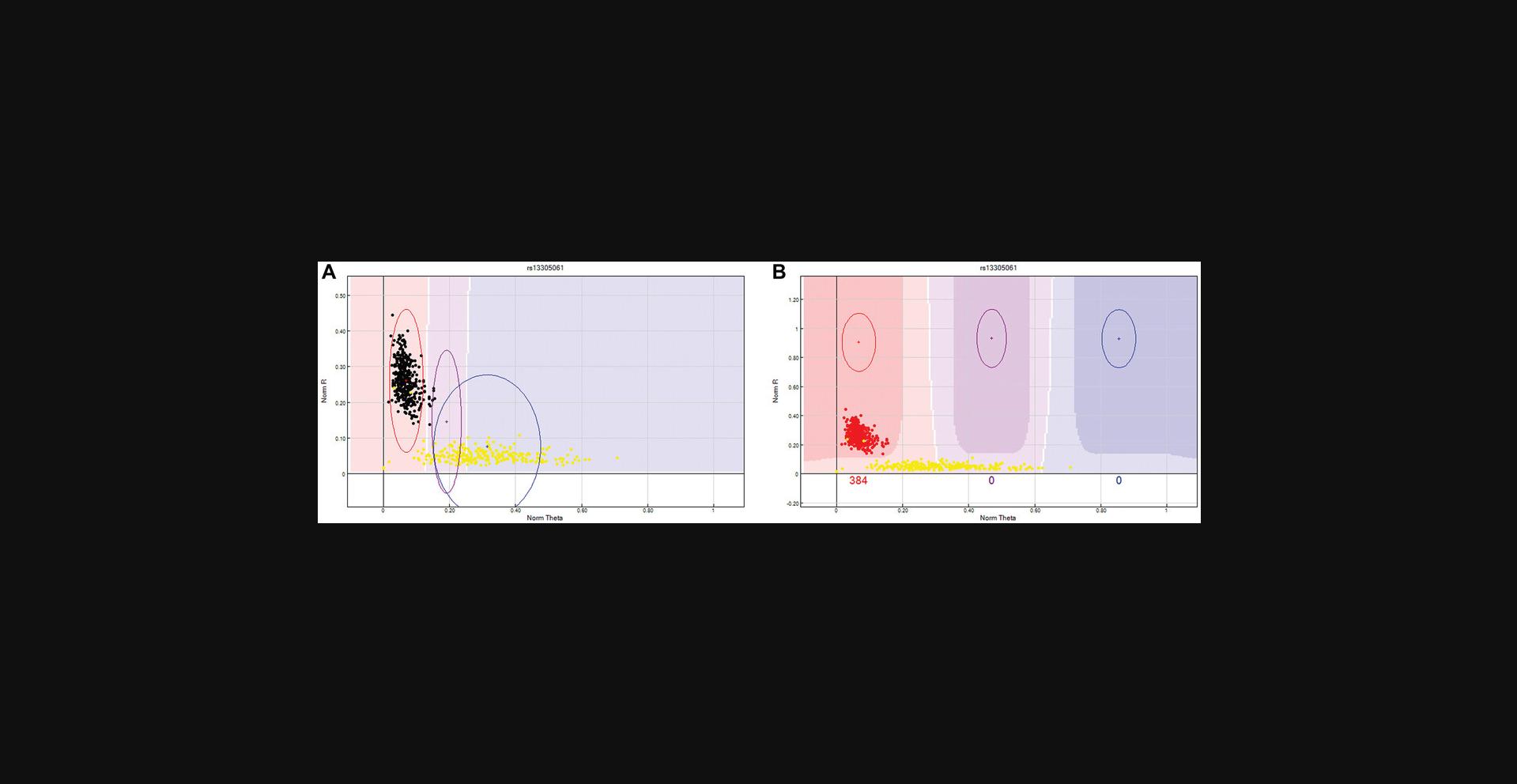
Now the Y chromosome SNPs can be processed. Female samples should not bind the Y chromosome probe, and as a result will exhibit a low binding intensity, which is represented in the “SNP Graph” with a low NormR intensity (<0.2). However, due to the repetitive nature of the Y chromosome and the fact that probe sequences are only 50 bp, probes targeting the Y chromosome may bind a different region of the genome, resulting in unusually high NormR intensity (>∼0.2). In the previous step, the female samples were highlighted to appear yellow within the SNP Graph pane. Using this color differentiation between males and females, the Y chromosome SNPs are processed. From the “SNP Table”, scroll through all Y chromosome SNPs and use the following criteria to manually re-cluster or zero any unreliable Y chromosome SNP:Female samples are expected to have a NormR intensity <0.2. If female samples have an unexpectedly higher value, then the Y chromosome probe has most likely bound to a different region of the genome and therefore needs to be manually removed. An example is provided in Figure2.If female samples have been clustered and the NormR intensity is <0.2, manually remove these samples from the cluster. An example is provided in Figure3.No samples should be assigned to the AB Cluster.
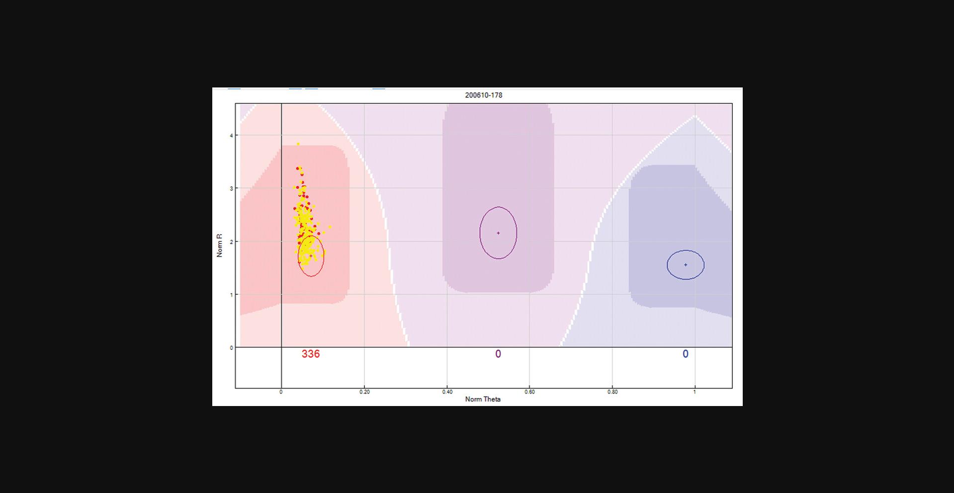
Y chromosome SNP with high female sample intensities. Y chromosome SNPs should not include female samples in any cluster. In this scenario, the female samples are highlighted in yellow and have intensities similar to the male samples (red dots). Given the repetitive nature of the Y chromosome and the fact that probe sequences are only 50 bp, this Y chromosome probe has most likely bound to a different region of the genome, and is, therefore, an unreliable SNP and should be removed.
13.Quality control of X chromosome.
Males have a single X chromosome; therefore, X SNPs should have no male subjects in the heterozygote cluster (AB). From the “SNP Table”:
-
From the “SNP Table”:Select the “Clear filter” button to remove any predefined filters.Click the “filter rows” button > select “Chr” from the Columns sub-window > select the operation “=” > enter the value “X” (this is case sensitive) > Click the “→” tab > click “OK”.Arrange SNPs by descending AB Frequency by selecting the “AB Freq” column followed by the “sort column (descending)” tab.Review these SNPs and ensure that no Male sample is assigned to the heterozygote (AB) cluster. If the male samples cannot be manually removed from the heterozygote cluster, then the SNP should be zeroed. An example is provided in Figure4.
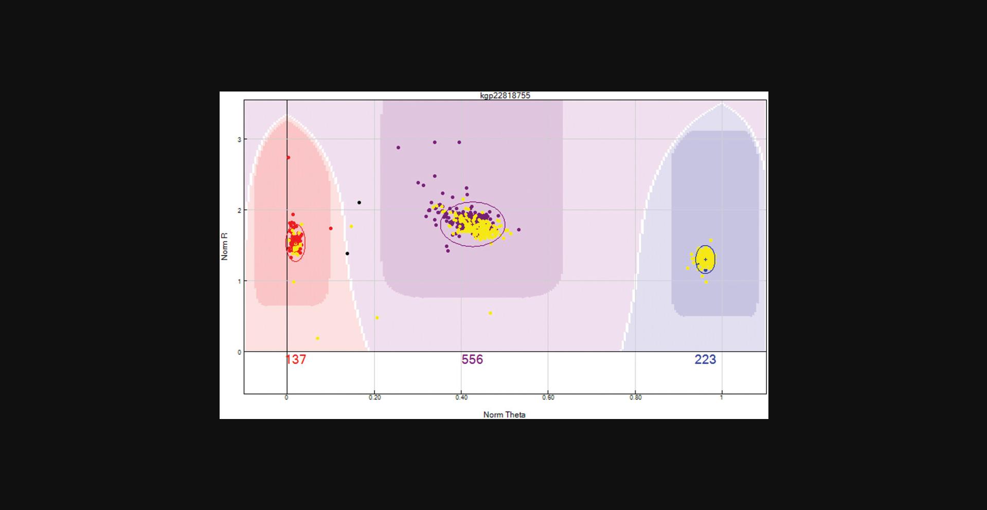
X chromosome unreliable SNP. This X chromosome SNP has female samples highlighted in yellow and male samples are red, purple, or blue depending on their clustering location. Male samples have a single X chromosome and therefore cannot be heterozygote as shown above. If the male samples cannot be manually removed from the heterozygote cluster, then the SNP should be zeroed.
14.Quality control of MT chromosome.
The MT chromosome is maternally inherited and should not show any heterozygote clusters.
-
From the “SNP Table”:Select the “Clear filter” button to remove any predefined filters.Use the “filter rows” button to select only MT chromosome SNPs and arrange by descending AB Frequency by selecting the “AB Freq” column followed by the “sort column (descending)” tab. Manually review all SNPs, ensuring there are no heterozygote clusters.
15.Quality control of XY chromosome.
The XY SNPs are known as the Pseudo autosomal (PAR) SNPs, and are present on both X and Y chromosomes; therefore, these SNPs may show male heterozygotes. There is no specific QC process for XY SNPs, and these should be processed along with the autosomal chromosomes.
16.Quality control of autosomal chromosomes.
The following steps will identify unreliably clustered SNPs that require manual reviewing and validation. Since the X, Y, and MT chromosomes have already been reviewed, these SNPs should be excluded from all the following filters; however, the XY chromosomes can be processed along with the autosomal chromosome. The following filters are all applied from the “SNP Table” window by selecting the “Filter Rows” tab. Some filters need to be selected from the “Sub Columns” window (within the “Filter Rows” option), which can be activated by selecting the chip name (usually 3rd last selection) in the “Columns” window.
-
Exclude the X, Y, and MT chromosomes. This filter should remain active when applying the autosomal chromosome filters. From the “SNP Table”:Use the “filter rows” button to select “Chr != X” and “Chr != Y” and “Chr != MT”. Click “OK”.
-
Review all SNPs that have failed to cluster:Use the “filter rows” button to add an additional filter where the “Call Freq = 0”. These SNPs have failed to cluster. Review these SNPs to see if any can be rescued by manual reclustering.
-
Review low-intensity SNPs. Remove the previous filter and individually add the following filters to identify SNPs with unexpected low intensities (example provided in Fig.5). Review SNPs after each filter, remove, and then add the next filter.Use the “filter rows” button to select “AB Freq != 0” and select the chip name from the “Columns” window to activate the “Sub Columns” window. Then, from the “Sub Columns” window, select “AB R Mean”, and select operation “<” and value “0.2”.Remove the previous filter. Use the “filter rows” button to select “AA Freq != 0” and select the chip name from the “Columns” window to activate the “Sub Columns” window. Then, from the “Sub Columns” window, select “AA R Mean”, and select operation “<” and value “0.2”.Remove the previous filter. Use the “filter rows” button to select “BB Freq != 0” and select the chip name from the “Columns” window to activate the “Sub Columns” window. Then, from the “Sub Columns” window, select “BB R Mean”, and select operation “<” and value “0.2”.
-
Review clusters that are closer to neighboring clusters than expected. Occasionally, clusters will be overlapping. If the clusters cannot be separated, then these SNPs should be zeroed. An example is provided in Figure6.Remove the previous filter. Use the “filter rows” button to select “Cluster Sep < 0.35". The data can be arranged by selecting the sort by ascending the “Cluster sep” column to have the SNPs with most likely overlapping clusters at the top of the table.
-
Review unusual levels of samples in the heterozygote (AB) cluster (Figs.7and8). Remove the previous filter, individually add the following filters, and review the filtered SNPs.Use the “filter rows” button to select “AB frequency > 0.6”. This will identify SNPs with excess samples in the heterozygote cluster.Use the “filter rows” button to select “AB frequency = 0 and minor allele frequency > 0”. This will identify SNPs with a lack of samples in the heterozygote cluster.Use the “filter rows” button to select “AA frequency = 1 and Call Freq < 1”. This will identify missed AB calls. If the number of SNPs to review is high, then call Freq can be reduced to a large value such as Call Freq = 0.98.Use the “filter rows” button to select “BB frequency = 1 and Call Freq < 1”. This will Identify missed AB calls. If the number of SNPs to review is high, then call Freq can be reduced to a large value such as Call Freq = 0.98.Use the “filter rows” button to select “Het excess > 0.3”. This will identify SNPs with excess samples in the heterozygote cluster to the expected Hardy-Weinberg Equilibrium.Use the “filter rows” button to select “Het excess < -0.3”. This will identify SNPs with a lack of samples in the heterozygote cluster to the expected Hardy-Weinberg Equilibrium.
-
Review SNPs where their clusters are outside their expected theta position (Fig.9). Remove the previous filter and individually add the following filters and review the filtered SNPs.Use the “filter rows” button to select “AA theta mean >0.3 and AA Freq !=0”.Use the “filter rows” button to select “BB theta mean <0.7 and BB Freq !=0”.Use the “filter rows” button to select “AB theta mean <0.3 and AB Freq !=0”.Use the “filter rows” button to select “AB theta mean >0.7 and AB Freq !=0”.
-
Review unusually large clusters (Fig.10). Remove the previous filter and individually add the following filters and review the filtered SNPs.Use the “filter rows” button to select “AA theta deviation >0.025”.Use the “filter rows” button to select “AB theta deviation ≥0.07”.Use the “filter rows” button to select “BB theta deviation >0.025”.
-
Review SNPs where the GenomeStudio algorithm has low confidence in clustering. The GenTrain score ranges from 0-1 where high values indicate high confidence in clustering.
Remove the previous filter and use the “filter rows” button to filter SNPs with “GenTrain scores of <0.7 and Edited !=1”. The edited column records SNPs that have been manually edited. In this filter, manually edited clusters are excluded from the filtered list.
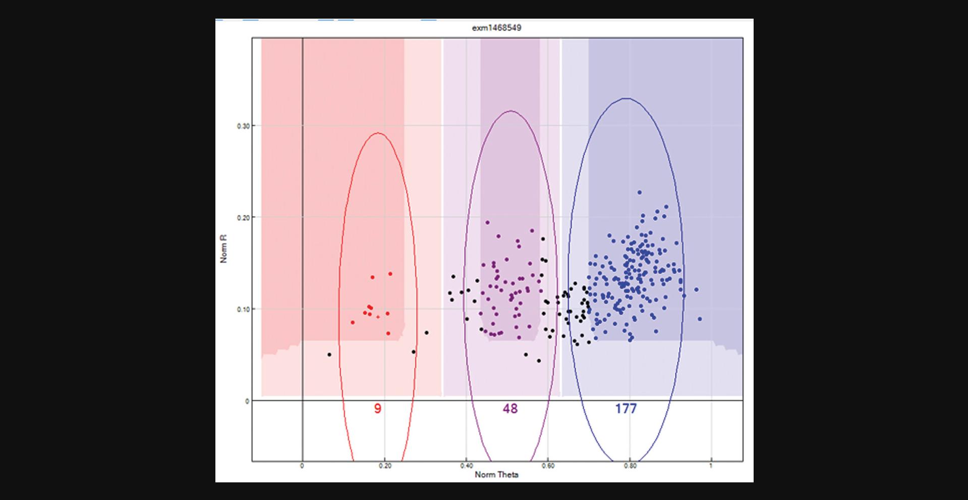
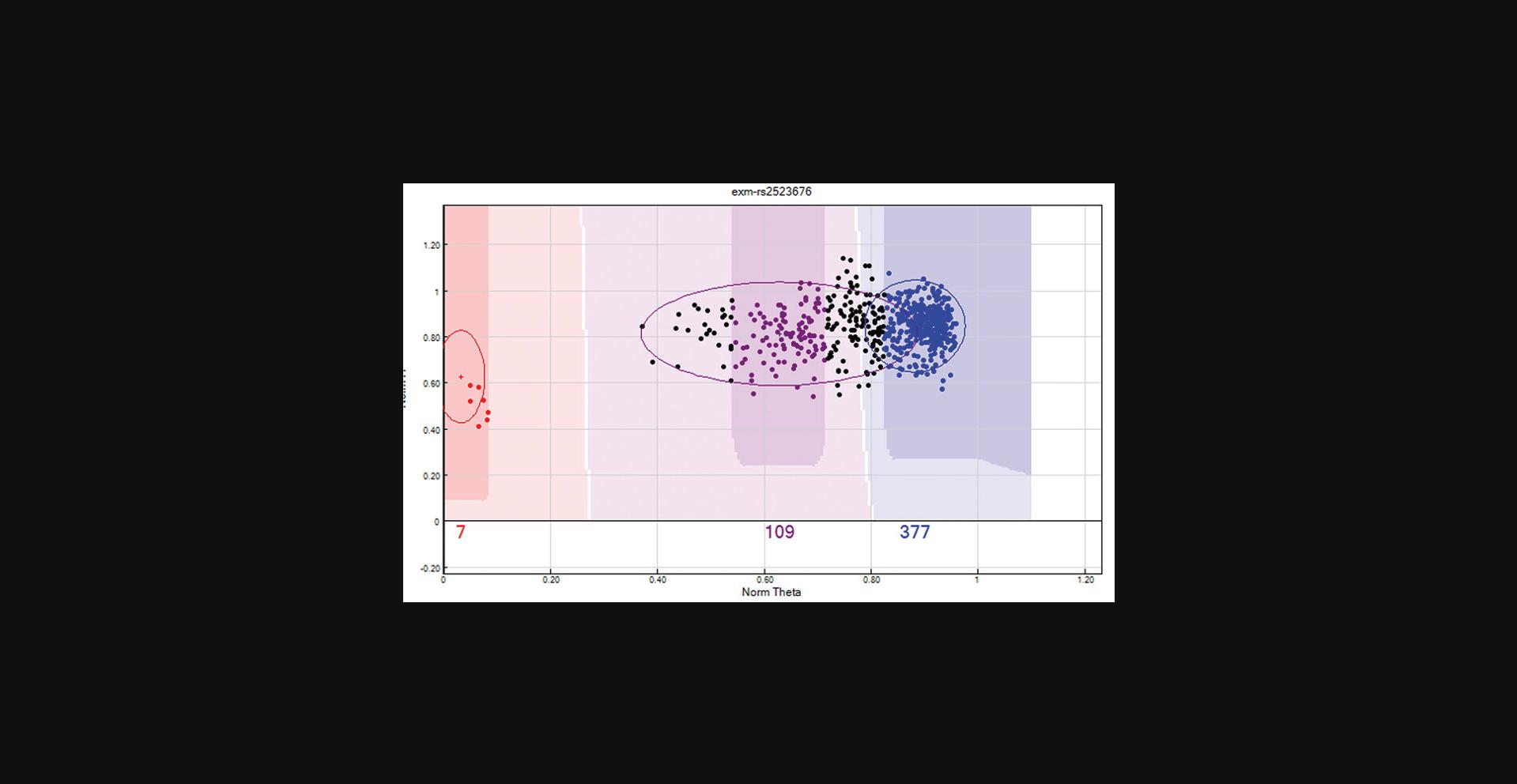
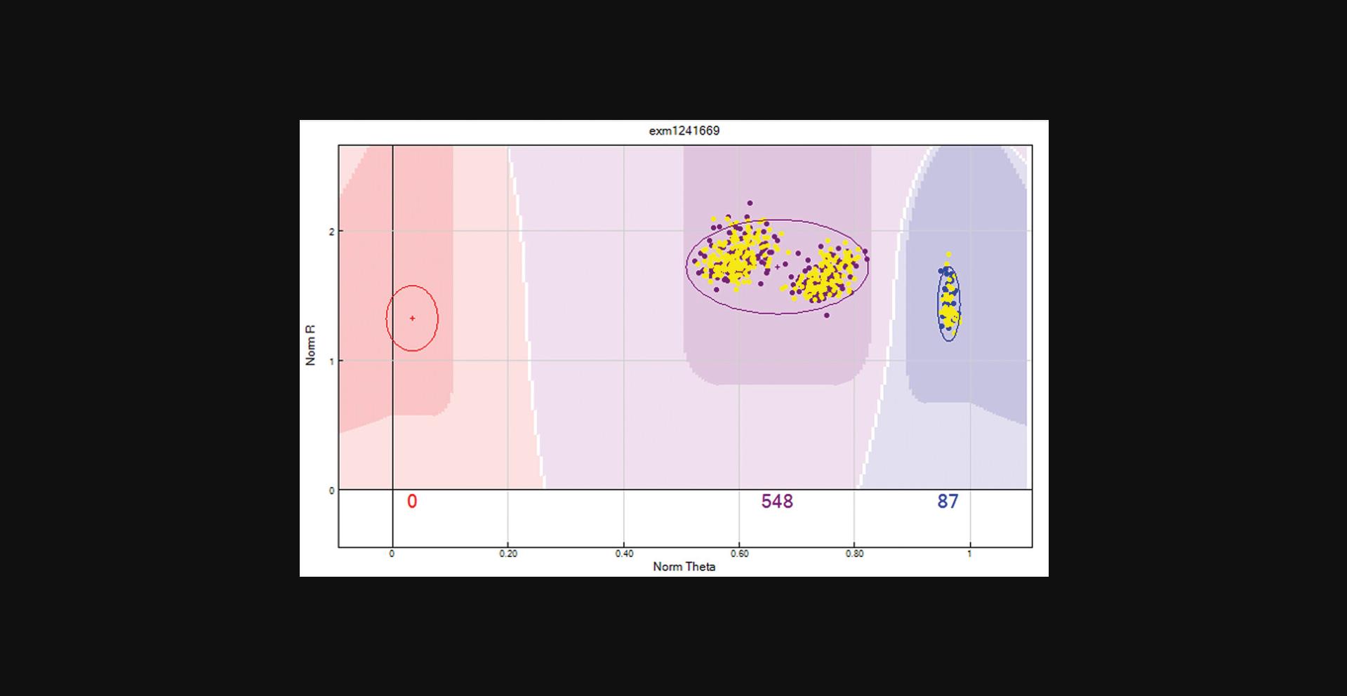
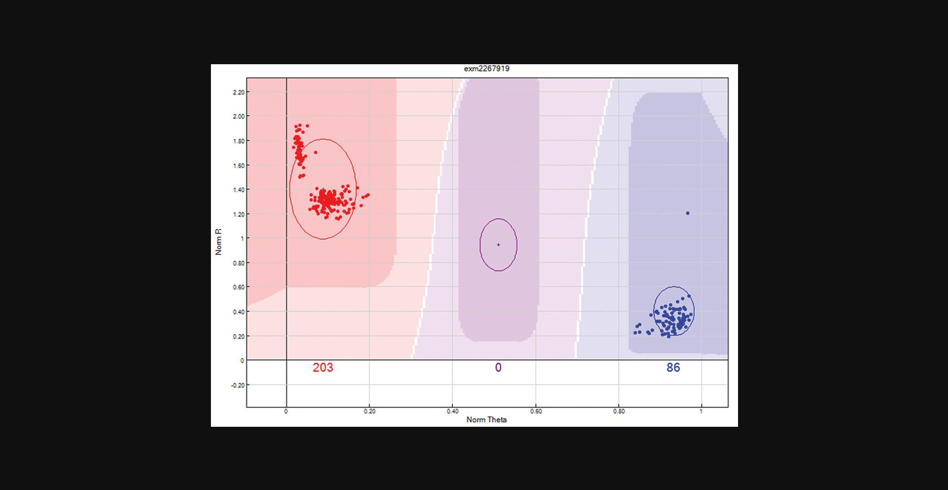
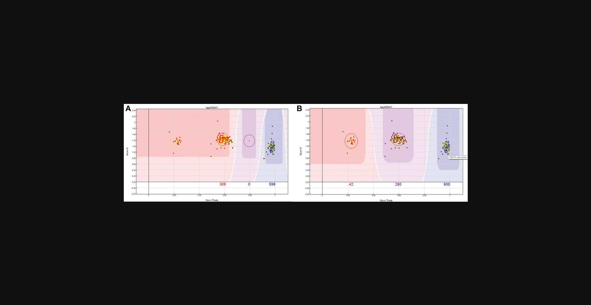
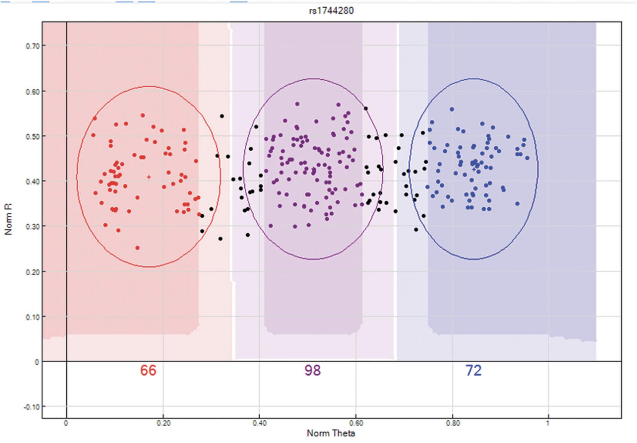
17.Quality control of replicated samples.
Samples can be replicated across batches for various reasons. GenomeStudio can identify discrepancies in SNPs between replicated samples and can flag them for the user to review. This can be extremely useful to identify batch effects or unreliable SNPs. Replicated samples are specified in the sample sheet, under the “replicate” column when loading data. However, users can specify these samples during QC by:
-
From the main window, select “Analysis” > “Edit Replicates”, select the replicate samples under the “Sample_ID1” and “Sample_ID2” sub-windows, and then click “Add”. Once all replicates have been added, click “OK” and GenomeStudio will update the statistics.
Discrepancies in replicated samples will be indicated by a square box in the “SNP Graph” window (Fig. 11). To QC based on replicate samples:
- b.From the “SNP Table”, remove all previous filters and use the “filter rows” button to filter SNPs with “Rep errors = “.
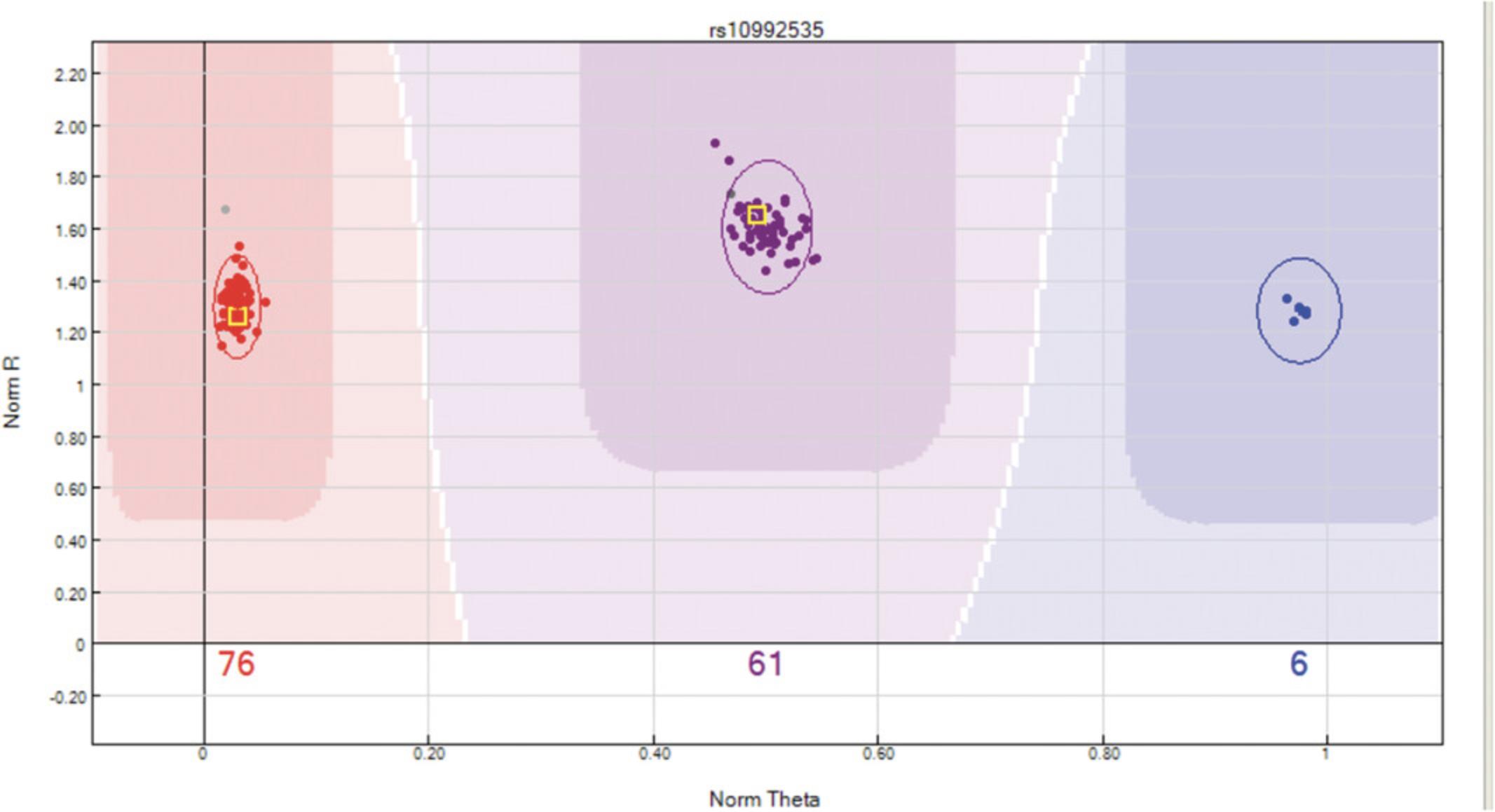
18.Quality control of parent-child samples.
Similar to replicated samples, parental information can be entered into the sample sheet when loading data into GenomeStudio or can be specified in GenomeStudio once a project has been created as follows:
-
From the main window, select “Analysis” > “Edit Parental Relationships” and select the appropriate samples under “Parent 1”, “Parent 2”, and “Child” sub-windows. Click “Add” and then click “OK”.
Discrepancies in parent-child (P-C errors) or parent-parent-child (P-P-C errors) will be indicated by a small “O” and “X” in the “SNP Graph” window, where “O” represents the parent and “X” represents the child. (Fig. 12). To QC based on relationship:
- b.From the “SNP Table”, remove all previous filters and use the “filter rows” button to filter SNPs with “P-P-C errors =1”, or if only one parent information is available, then filter by “P-C errors = 1”.
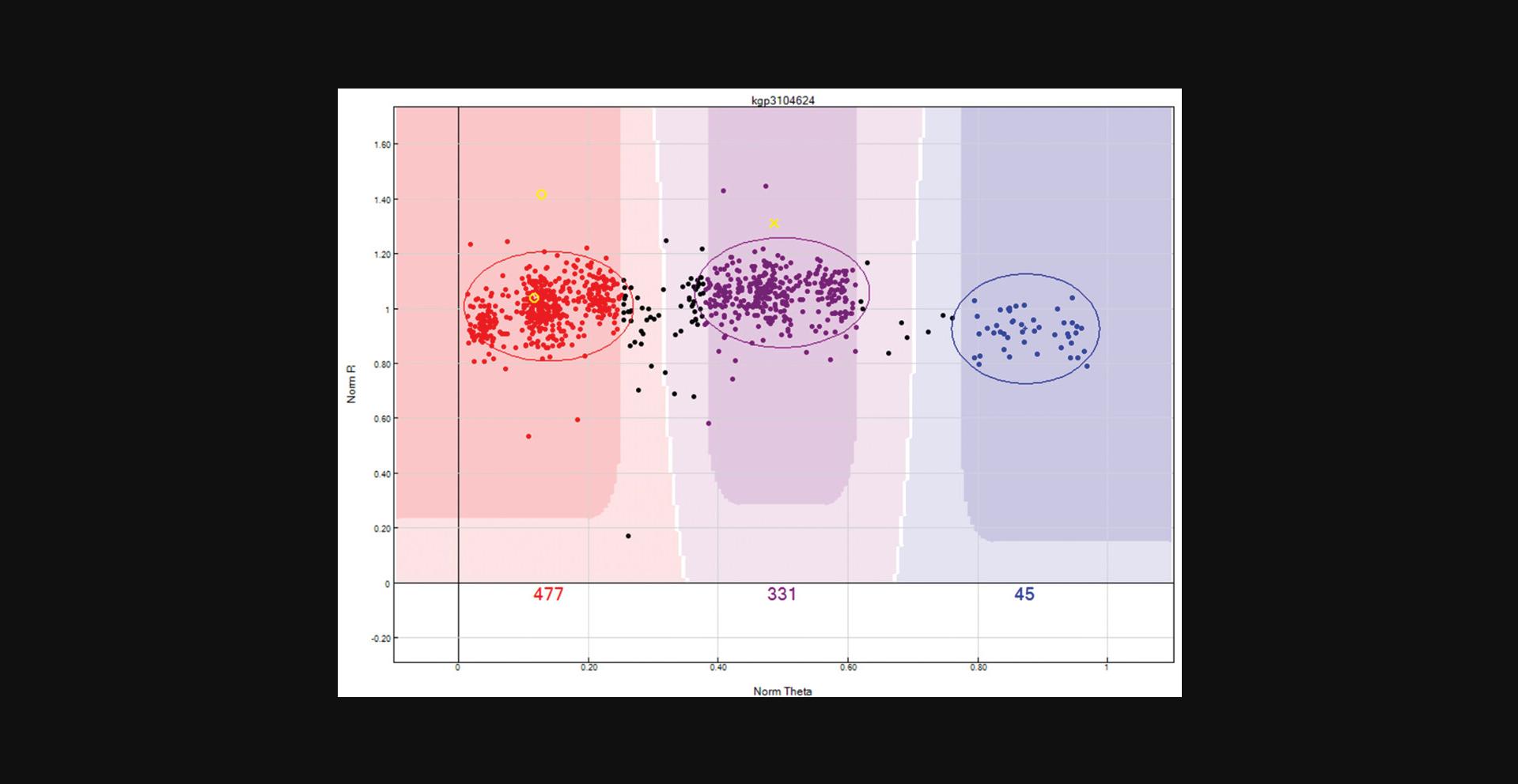
19.Predicting gender for samples.
GenomeStudio uses the X chromosome to estimate the gender of samples. Therefore, the gender of samples should only be predicted after processing the X chromosome:
-
From the “SNP Table”:Select “Clear filter”.Click the “Select all” button to highlight all SNPs, right-click, and “Update Selected SNP Statistics”.
-
From the “Samples Table”:Right-click and “Recalculate Statistics for all Samples”.Click the “Select all” button to highlight all samples, right-click, and select “Estimate Gender for selected samples”. When prompted “populate Gender column”, select “No”.Select the “Column Chooser” icon and show “Gender Est” from Hidden Columns.
20.Updating statistics.
Following QC, the statistics for samples and SNPs should be updated. This step can be skipped if the gender was predicted in the previous step, as the gender prediction process incorporates updating statistics. To update statistics:
-
From the “SNP Table”:Click “Select all”.Right-click on the highlighted SNPs.Click “Update Selected SNP Statistics”.
-
From the “Samples Table”:Click “Select all”.Right-click on the highlighted samples.Click “Recalculate Statistics for all Samples”.
21.Saving cluster positions.
Once a project has been processed, the cluster positions for the SNPs can be exported and used to process the next batch or a new project. This can significantly reduce the time required for QC. However, it is recommended to merge and process batches together, as more samples lead to clearer and more well-defined clusters. Nevertheless, this process can be used to process different batches or projects that have been genotyped on the same genotype array (including version number).
To export the cluster positions:
-
From the main window, click “File” → “Export Cluster Positions” → “For all SNPs”.
-
Select a location to store the cluster file (.egt) and save.
This file can be used to cluster new data that have been genotyped on the same genotyping array. When creating a new genotyping project, check the “Import cluster positions form a cluster file” box and specify the cluster file (.egt) location when prompted. This is further detailed in this protocol under step 2, “Creating a new genotyping project”.
22.Saving project.
It is strongly advised to save changes to the project while QC is ongoing and after QC has finished.
-
From the main window, click on “File” → “Save Project Copy As”.
-
Under “projects Repository”, browse to the location where you would like to save the data.
-
Under “Project Name”, create a name for the project. Keeping in line with the naming convention used to create the project, we recommend using[PROJECT_NAME]_[DATE]_02.bsc, where the “02” indicates processed data.
-
Click “OK”.
23.Creating input file format for COPILOT container.
The COPILOT container will automate a series of bioinformatics analyses that will apply a secondary clustering algorithm to improve data quality, while also identifying potential issues with the data. The following steps will generate the required input format from GenomeStudio:
-
Remove all filters from the “Samples Table” and the “SNP Table”.
-
Select the “Full Data Table” tab.
-
Select “Column Chooser”.
-
From the “Displayed Columns” window select:IndexAddressGen Train ScoreFrac AFrac CFrac GFrac T
-
Click Hide.
-
From the “Displayed Subcolumns” window select:ScoreThetaR
-
Click Hide
-
From the “Hidden Subcolumns” window select:XY
-
Click Show.
-
Ensure that the columns are in the order as illustrated in Table1.
-
Click the “Select all” icon to highlight all the SNPs.
-
Click the “Export displayed data to file” icon.
-
Browse to a location where you want to save the data, and save as[PROJECT_NAME]_[DATE]_intensity_data.reportin tab-delimited format.
24.Creating PLINK data (optional).
Users can generate PLINK-formatted data directly from GenomeStudio and follow guidelines in Coleman et al. (2016) to perform a typical GWAS analysis. However, it is strongly advised to generate the COPILOT output format data as described above and further process the data through the COPILOT container to further increase data quality. Nevertheless, if users would like to generate PLINK-format data at this stage, then:
-
Download and install the PLINK plugin from the GenomeStudio website (version used in this protocol is v2.1.4) athttps://support.illumina.com/downloads/genomestudio-2-0-plug-ins.html.
-
From the main window, click “Analysis” > “Reports” > “Report Wizard”.Click “Custom Report” and select “PLINK InputReport 2.1.4 by Illumina, Inc. from Illumina, Inc.”.Users are then provided with options on how to handle repeated samples (if present) by either selecting best sample by GC Score or assigning unique IDs to each sample.If multiple sample groups are available and have been specified in the sample sheet, GenomeStudio will provide an option to export by sample group. Select the group you would like to export and click “Next”.Next, users are provided options on how to handle zeroed samples. They can be removed at this stage or users can have them exported into the PLINK file with a zero call rate. We recommend removing these zeroed samples at this stage to lower the computational burden.This is followed by the options on how to handle zeroed SNPs. Similar to zeroed samples, we recommend removing these zeroed SNPs to lower the computational burden.Select the “Output Path” and provide a name in the “Report Name”, then Click “Finish”.
| Name | Chr | Position | Sample 1 | Sample 2 | … | ||||
|---|---|---|---|---|---|---|---|---|---|
| G Type | X | Y | G Type | X | Y | … | |||
Basic Protocol 2: COPILOT: A CONTAINERISED WORKFLOW FOR PROCESSING ILLUMINA GENOTYPING DATA
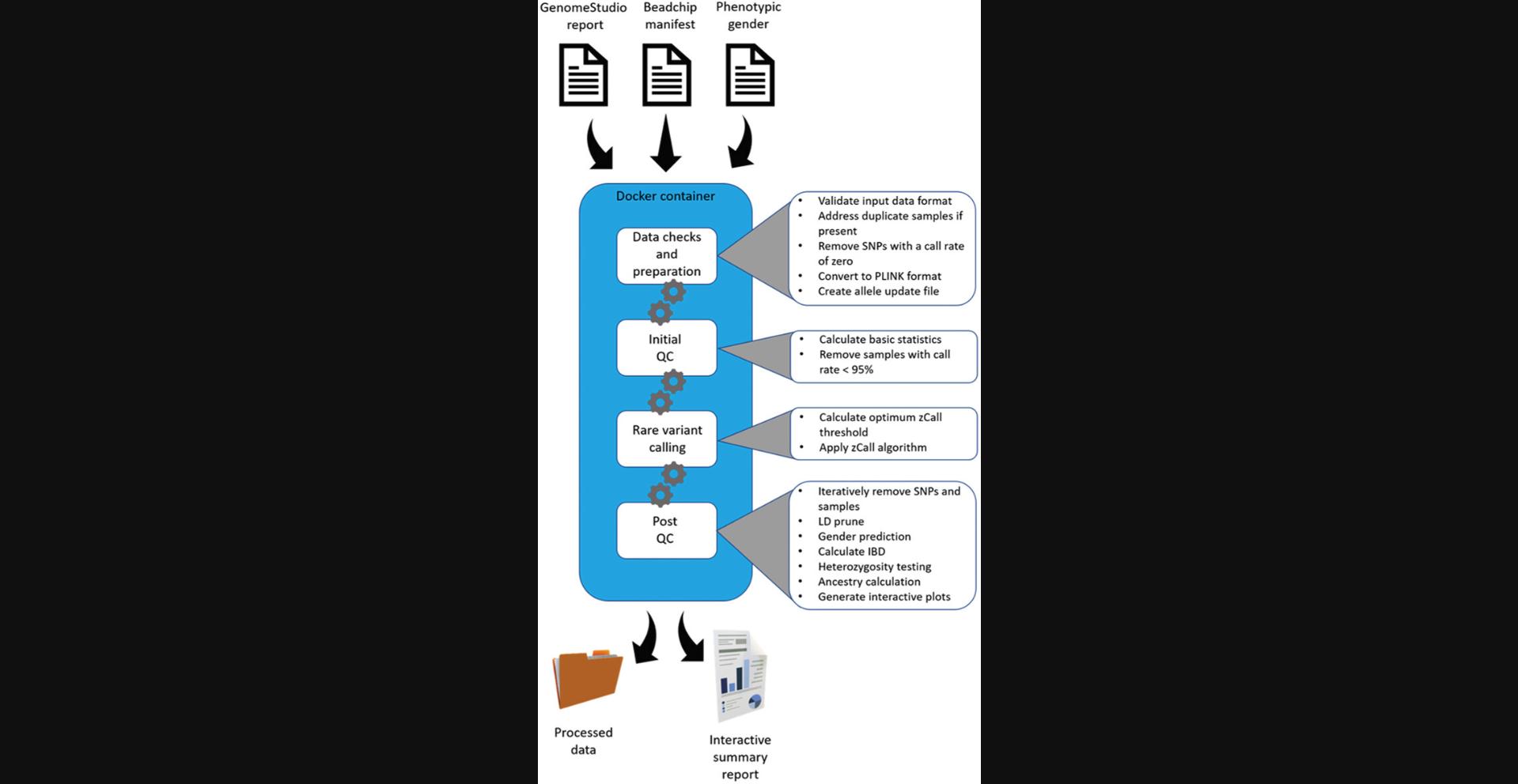
This protocol deploys a containerized workflow (COPILOT) that will effortlessly further process genotype data that has been pre-processed in GenomeStudio. The COPILOT container starts by performing pre-analysis checks of the input data, calculates basic statistics, and prepares for the zCall rare variant–calling algorithm. The zCall caller is an established software (Goldstein et al., 2012), which attempts to assign genotype calls to SNPs that have been missed by the GenomeStudio GenCall algorithm, which commonly represent the rare variants. This process essentially increases the overall sample call rates, which effectively increases data quality. COPILOT then converts data to PLINK format and uses the manifest file to update all alleles in AB format to Illumina TOP strand, and then performs multiple analyses as recommended in Coleman et al. (2016). These include iteratively removing SNPs and samples to a user-defined threshold, pruning data for linkage disequilibrium (LD), and removing high regions of LD and non-autosomal regions, identifying potential sex discrepancies, calculating identity-by-descent (IBD), performing a heterozygosity test, and calculating ancestry of each sample based on the 1000 Genomes reference panel (Altshuler et al., 2012).
Genotyping data often consists of duplicate sample IDs, which can cause issues during data processing. COPILOT handles duplicate sample IDs by assigning temporary unique sample IDs to duplicate samples, allowing each duplicate sample to be independently treated during the data processing stage. The resulting processed data is provided back to the user in PLINK format, with any duplicate sample IDs reverted to the original ID, but with a record kept for users to re-identify them if required. An outline of the COPILOT process is provided in Figure 13.
Necessary Resources
Hardware
- CPU Speed–2.0 GHz or greater
- Processor–64-bit, with 2 or more cores
- Memory–8 GB or more
- Hard Drive–100 GB or larger
- Operating System–Linux or Windows or macOS
Software
- Docker
Files
- GenomeStudio output file as created in Basic Protocol 1.See Table 1. An example file is available at:
- Gender file: The gender file contains the gender for each sample in tab-delimited format. The file contains two columns with sample ID in the first column and gender information in the second column (no headers). For genders, M/Male must be used for male samples and F/Female must be used for female samples. If the gender is unknown for any reason, then the genders can be left blank or kept as “Unknown”. An example file is available at:
- Illumina manifest file: The Illumina manifest file (*.csv) contains details about the SNPs used for genotyping. This file is used to update the allele coding to Illumina TOP. Ensure that the manifest and project are in the GRCh37 (hg19) genome build, as the ancestry data is calculated based on these positions. The Illumina manifest file name should end in “A1”; if it ends in “A2” this is most likely the 38 build. An example file is available at:
- COPILOT container:
- The docker image is available at:
- COPILOT execution file:
- The file to run the docker image is available at:
1.Installing Docker.
Docker should be downloaded and installed as detailed on their website (https://docs.docker.com/get-docker/).
2.Importing the COPILOT container.
- a.Using a CLI, navigate to the folder where the docker image (COPILOT.tar) is stored and import the image into your docker repository:
- docker load -i COPILOT.tar
- b.Confirm the docker image has been correctly imported using:
- docker images
- c.Give the newly imported docker image a name, replacing the docker IMAGE ID (c0ae9d5736fc) with what you have listed. Ensure the new name provided is “COPILOT”, as the execution script will be looking for this image.
- docker tag c0ae9d5736fc COPILOT
- d.Confirm the docker image has been correctly renamed using:
- docker images
3.Running the COPILOT container.
-
Move the GenomeStudio report file, gender file, Illumina manifest file, and COPILOT execution script into the same directory.
-
Edit the “execution file” and specify:data_location: This is the location where the data is stored and where the output folders and files will be generated. Ensure you specify the full path of the folder.manifest_file: This is the name of the manifest file.clinical_gender: This will be the name of the clinical gender file.report_file: This will be the name of the GenomeStudio report file.sample_call_rate: Samples with a call rate below 95% are removed before processing the data through the rare variant calling algorithm, zCall (as recommended by the zCall protocol). To calculate potential problematic samples post zCall, such as sex discrepancies, heterozygote outliers, IBD, ancestry, etc…, an additional “sample_call_rate” threshold is applied. Samples below this threshold are only temporarily removed to identify problematic samples; they are re-introduced into the data at the end of the pipeline for the user. The recommended (default) value is set at 0.98. Only change from default if the data has a large number of samples with a low call rate below 0.98. Users can specify 0.95, 0.96, 0.97 or 0.98
-
Save changes to the script and run the execution script:bash COPILOT_execution.sh
-
The docker container will be running in the background. To view the progress of the container, the user can view the output folder or check the docker progress using:docker ps -a
-
Check the “QC_logfile.txt” file for any errors after the pipeline has finished.grep "error" QC_logfile.txt
GUIDELINES FOR UNDERSTANDING RESULTS
A customized and detailed report specific to the data being analyzed will be generated as a summary report. If the summary report fails to populate, then an error in the analysis has occurred and the error log should be carefully checked. All files generated throughout the analysis are provided to the user and organized in the following manner:
- 1.0.Scripts_and_logfiles : This contains the COPILOT execution script and associated log files
- 2.1.GenomeStudio_report_file : This contains the processed GenomeStudio output file that was used as input for the COPILOT QC Pipeline
- 3.2.Illumina_manifest_and_allele_update_file : This contains the Illumina manifest and the allele update files in the Illumina TOP strand format
- 4.3.Clinical_gender : This contains the clinical gender information
- 5.4.Prepare_report_file : This contains a modified report file with problematic samples removed
- 6.5.Duplicate_samples : This contains information duplicate IDs identified and any associated changes
- 7.6.Samples_SNPs_removed : This contains a list of samples and SNPs removed before applying the zCall algorithm
- 8.7.zCall : This contains all zCall-related files
- 9.8.FINAL_QC_DATA : This contains the final processed data after zCall. The data is provided in the Illumina TOP strand. If duplicate samples existed in this data, then the “.fam_with_dup_ID” contains sample IDs that were changed. This data should be used for further analysis
- 10.9.Additional_QC : Contains additional processing that was performed on the final processed data to identify additional potential problematic issues
- a. 1.Low_call_rate_SNP_samples_removed : This contains the PLINK binary file when SNPs with a call rate below 95% and samples with a call rate below the user-defined threshold (default is 98%) are removed. The “08.zcall_final_low_snp_sample_removed.mindrem.id” file lists the samples removed
- b. 2.Pruned_data : This contains the pruned data
- c. 3.Sex_check : This contains gender-related information and plots. The “08.gender_missmatches.txt” file lists all samples with gender mismatches
- d. 4.Heterozygosity_test : This contains heterozygosity test related files and plots. The “08.zcall_final_highLD_and_nonautosomal_removed.het.LD_het_outliers_sample_exclude.txt” file lists all samples identified as outliers
- e. 5.Identity-by-Descent : This contains IBD related files and plots. The “08.IBD_outliers.txt” file contains samples identified as related
- f. 6.Ancestry_estimation : This contains files and plots relating to ancestry check
- g. 7.Call_rate_plots : This contains sample call rate plots after QC
- h. 8.MAF_plot_and_snp_summary : This contains MAF plots and summary on number of SNPs
- i. 9.Compiled_list_of_potential_problematic_samples : This contains a list of samples that have been identified as outliers
- 11.summary_report.html : This is an interactive summary report which provides more information on the data.
Throughout the data processing pipeline, only SNPs deemed unreliable in GenomeStudio and samples with a call rate below 95% were removed from the data. The list of samples removed (if any) can be found in the “6.Samples_SNPs_removed“ folder. The remaining SNPs and samples were further processed using zCall to create the “final processed data“ which is located in the “8.FINAL_QC_DATA“ folder. Additional SNPs and samples (SNPs <95% and samples <98%) were only removed to calculate the gender mismatches, heterozygosity, related samples, and ancestry statistics. These SNPs and samples have been reintroduced in the “final processed data“, but a list of these samples is provided in the “9.Compiled_list_of_potential_problematic_samples” folder. If conducting a GWAS study, the “final processed data“ can be analyzed using the recommended guidelines detailed by Coleman et al. (2016), who also provides a GWAS codebook.
COMMENTARY
Background Information
The COPILOT protocol provides an in-depth and clear guide to processing raw Illumina genotype data in GenomeStudio, followed by a containerized workflow to automate an array of complex bioinformatics analyses to improve data quality and to identify typical GWAS data issues. The COPILOT protocol is currently deployed in the King's College London's (KCL) Institute of Psychiatry, Psychology and Neuroscience's (IoPPN) Genomics & Biomarker Core Facility, and has been successfully used to process thousands of samples on various genotyping chips, including the Infinium Core, Exome, CoreExome, OmniExpress, Omni2.5, Omni5, PsychArray, Multi-Ethnic, Global Screening Array range, and H3Africa Consortium arrays. The container takes approximately 60 min to process ∼300 samples on the Infinium HumanCoreExome Array (∼550,000 SNPs) using a machine with six dual cores and 32 GB RAM. A substantially larger project with ∼500 samples on the H3Africa Consortium Array (∼2.3 million SNPs) takes approximately 30 hr to process.
Sample quality improvement–case study
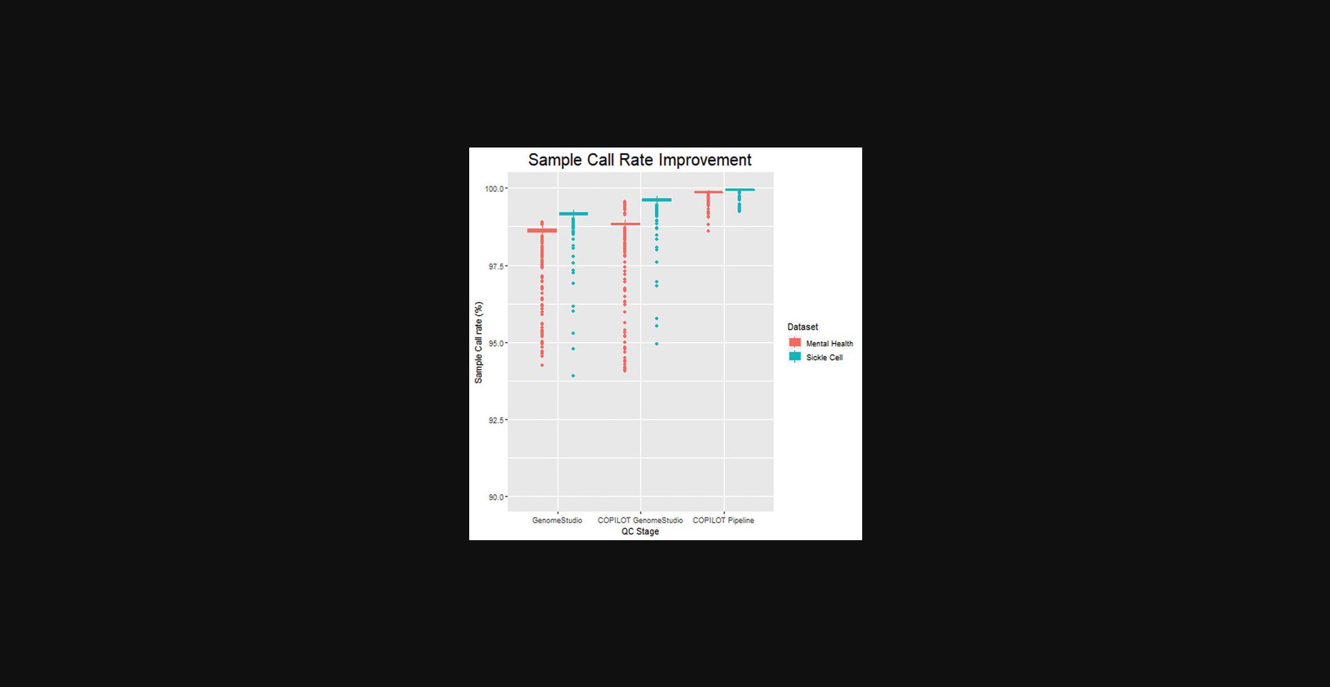
The sample call rate is the fraction of the SNPs with a genotype call for a given sample, with higher sample call rates indicative of better sample quality. The COPILOT protocol was applied to 3270 samples from two different cohorts using two different Illumina genotyping arrays. The first cohort is a mental health disorder consisting of 2791 samples collected as either blood, buccal swab, or saliva, and genotyped using the Infinium Global Screening (GSA) array with Multi-disease (MD) drop-in (∼750,000 markers). The second cohort is a sickle cell cohort consisting of 479 samples collected as blood samples and genotyped using the Infinium H3Africa Consortium array (∼2,200,000 markers).
The cohorts were independently processed in GenomeStudio using the default GenCall clustering algorithm with extreme outliers removed (samples with a call rate below 90%). An initial average sample call rate of 98.55% (95% CI 98.58-98.67%) was achieved for the mental health cohort, and 99.19% (95% CI 99.14-99.22%) was achieved for the sickle cell cohorts before any QC. Following the COPILOT QC protocol (including GenomeStudio QC and COPILOT container) and without requiring removal of additional samples, the average sample call rates improved to 99.86% (95% CI 99.86-99.89) and 99.93 (95% CI 99.93-99.95), respectively, averaging an improvement of 1.24% across the 3270 samples. Notably, the sample call rates significantly improved for samples at the lower end of the sample quality spectrum (Fig. 14). The sample call rate threshold used to exclude samples from a typical GWAS varies, with 98% commonly used (Coleman et al., 2016). The mental health and sickle cell cohort consisted of 129 and 12 samples, respectively, where sample call rates were below 98%. The average call rates for these 141 samples were 96.6% (95% CI 95.6%-97.7%) before QC; however, following the COPILOT protocol, these 141 samples all attained a call rate above 98% and averaged 99.6% (95% CI 99.5%-99.7%), and therefore would have been rescued for further analysis.
Automated identification of problematic samples–case study
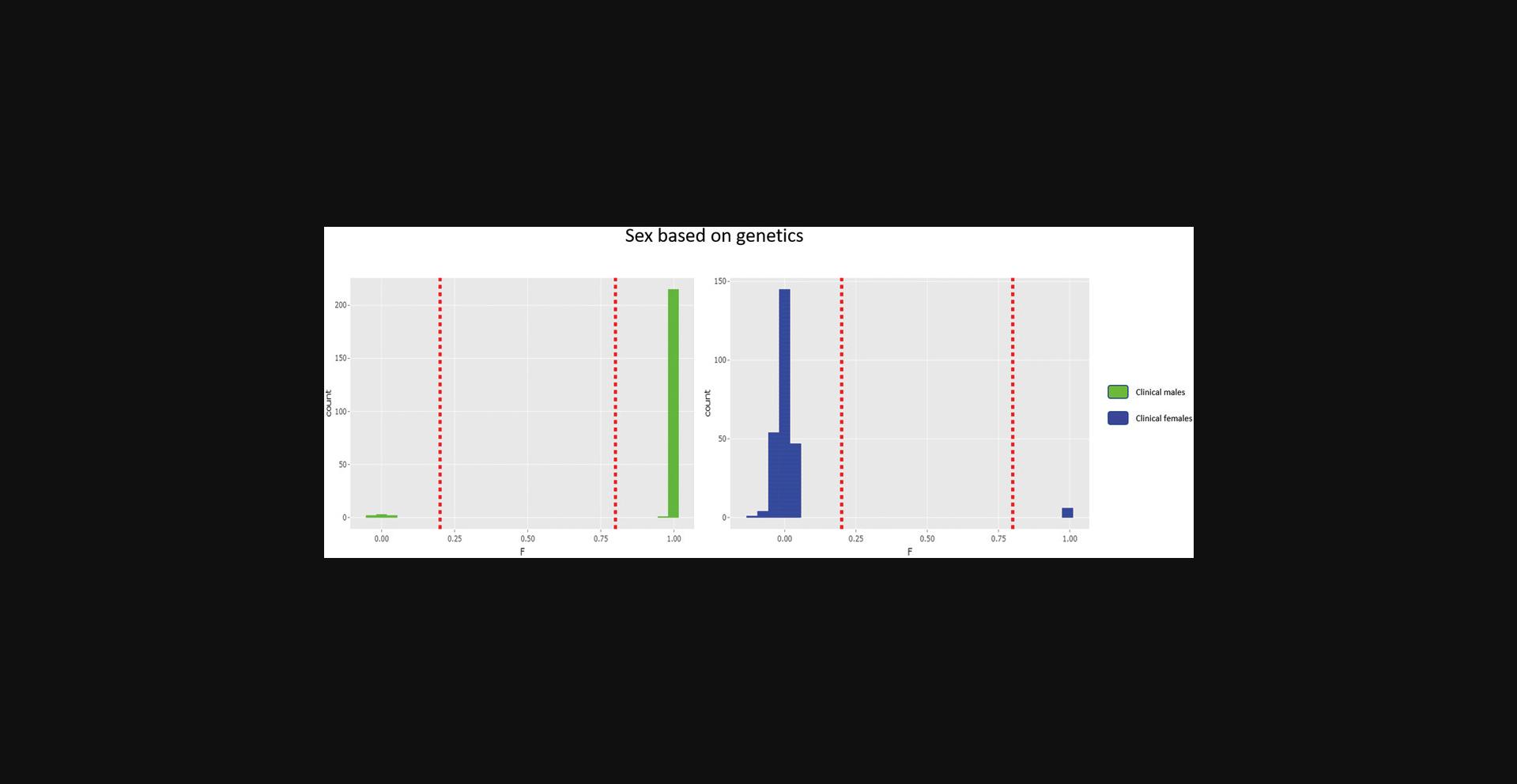
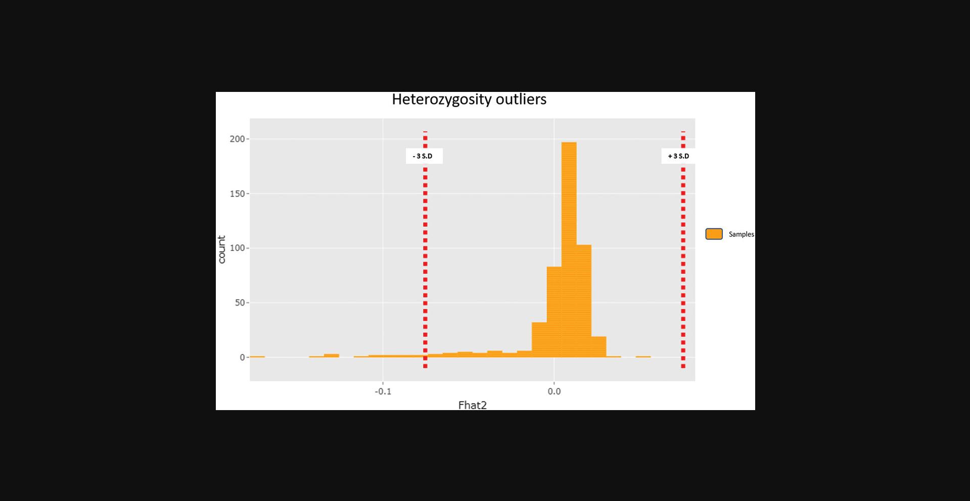
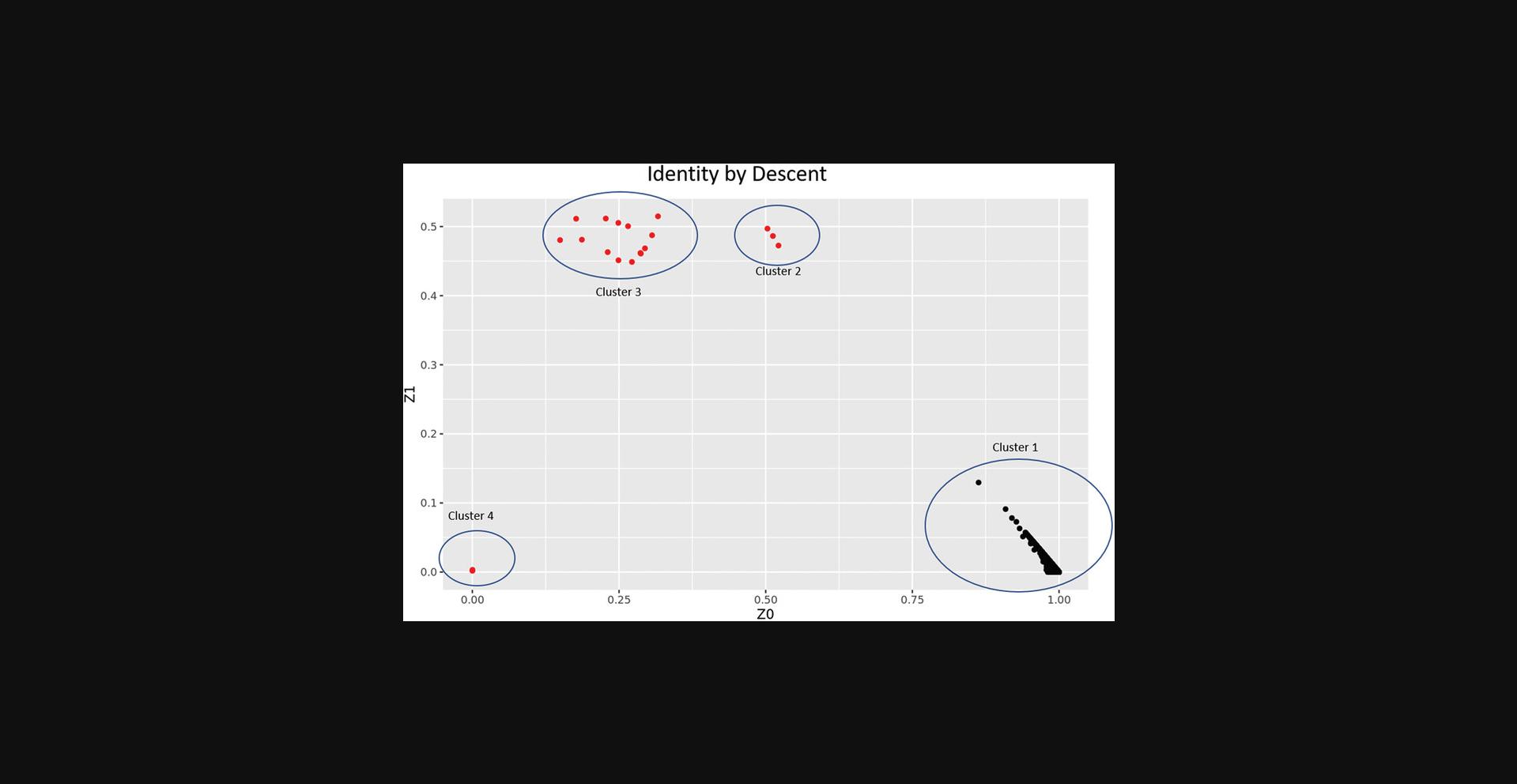
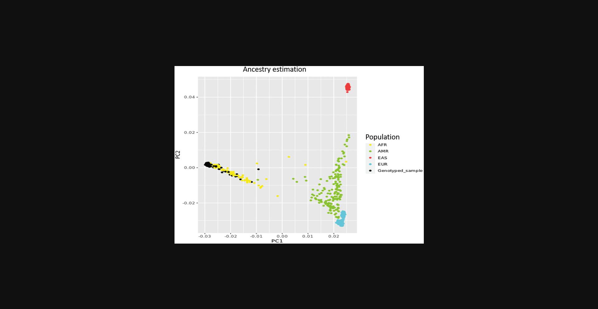
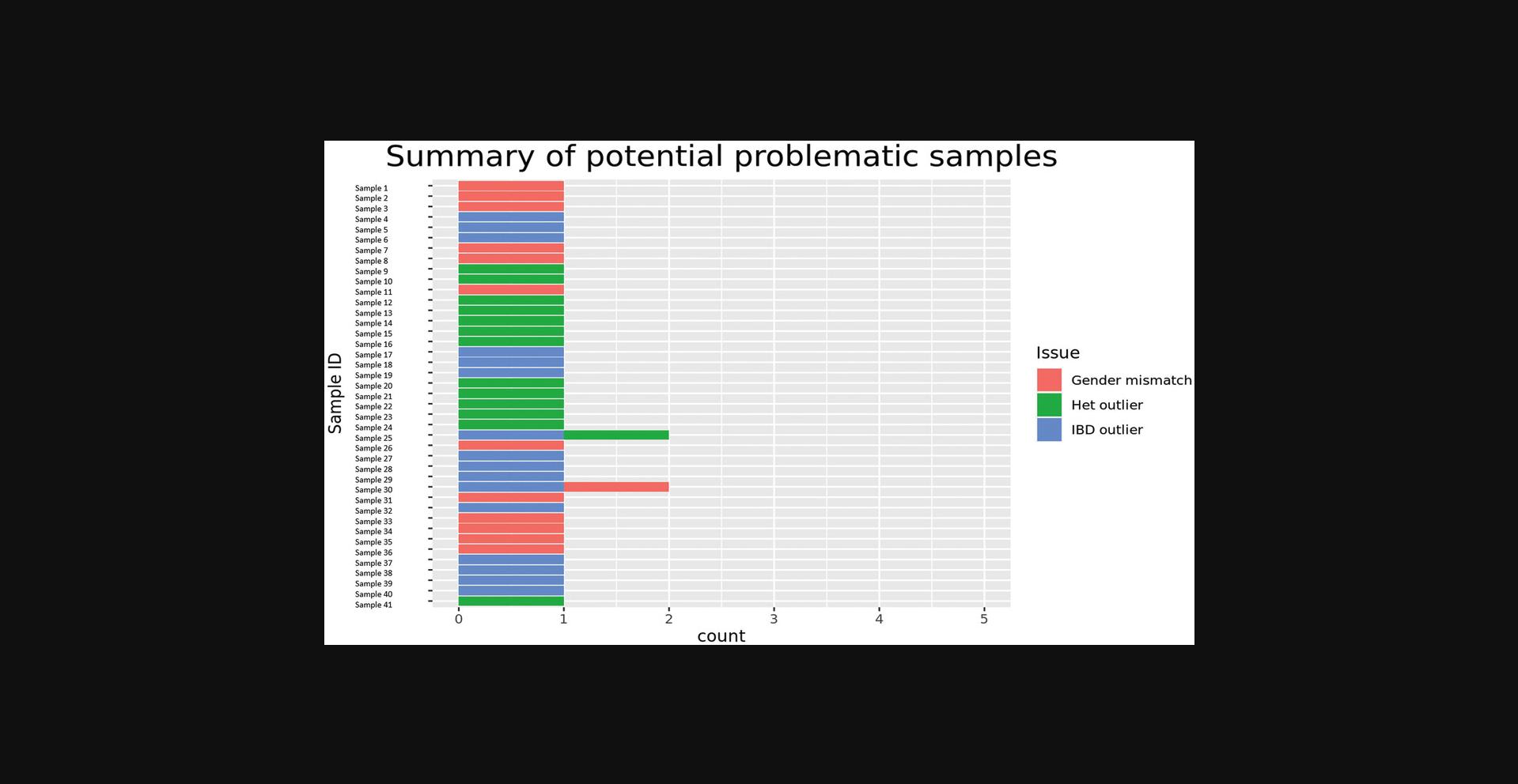
The COPILOT container automates the identification of potentially problematic samples for the typical GWAS and provides findings through an informative and interactive summary report (example provided here at https://khp-informatics.github.io/COPILOT/README_summary_report.html). As an example, COPILOT was used to process the sickle cell cohort consisting of 479 patients. As a result, COPILOT identified genotypic and phenotypic gender discrepancies (Fig. 15), heterozygosity outliers (Fig. 16), related samples (Fig. 17), and sample ancestry based on the 1000 genome reference panel (Fig. 18), and provides an overall summary of potential problematic samples (Fig. 19).
Critical Parameters and Performance
There are no critical parameters that require adjustments. The complete COPILOT protocol can take a few days to a few weeks depending on the number of SNPs, samples, compute power, and user ability. The COPILOT container takes approximately 60 min to process ∼300 samples on the Infinium HumanCoreExome Array (∼550,000 SNPs) using a machine with six dual cores and 32 GB RAM. A substantially larger project with ∼500 samples on the H3Africa Consortium Array (∼2.3 million SNPs) takes approximately 30 hr to process.
Troubleshooting
The COPILOT protocol consists of two distinct stages. The first involves processing data through the Windows-based Illumina GenomeStudio software and the second involves a dockerized pipeline. The two most common problems occur when loading data. When loading data into GenomeStudio using the sample sheet, ensure that the full path to the IDAT data location is used in the “Path” column and the correct manifest for the project is specified, including the array version number. The next common problem occurs when running the COPILOT container. The container will check that the manifest is in build 37 and the GenomeStudio report file is in the correct file format prior to QC, and will not run if there is an error in either. The container also generates a logfile (“QC_logfile.txt”) in the newly created “0.Scripts_and_logfiles” folder, which will be located in the output folder the user specifies in the COPILOT “execution file”. The log file records all internal commands that are performed, including any errors that may have occurred. Users can “grep error QC_logfile.txt” to find any errors in the processing that may have occurred.
Maintenance
The QC pipeline has been dockerized to preserve the various analysis scripts and software applications in a contained environment, which is deployable on multiple operating systems. Theoretically, the dockerized container will not require any maintenance. However, new feature may be added and new releases of COPILOT may occur in the future, and therefore users are strongly advised to visit the COPILOT website at https://khp-informatics.github.io/COPILOT/index.html for any new releases and updates. If any user would like to see new features added or have technical questions, then please contact the authors.
Suggestions for Further Analysis
Throughout the data processing pipeline, only SNPs deemed unreliable in GenomeStudio and samples with a call rate below 95% were removed from the data. The list of samples removed (if any) can be found in the “6.Samples_SNPs_removed“ folder. The remaining SNPs and samples were further processed using zCall to create the “final processed data“, which is located in the “8.FINAL_QC_DATA“ folder. Additional SNPs and samples (SNPs <95% and samples <98%) were only removed to calculate the gender mismatches, heterozygosity, related samples, and ancestry statistics. These SNPs and samples have been reintroduced in the “final processed data“, but a list of these samples is provided in the “9.Compiled_list_of_potential_problematic_samples” folder. If conducting a GWAS study, the “final processed data“ can be analyzed using the recommended guidelines detailed by Coleman et al. (2016), which also provides a GWAS codebook.
Supplemental Files
An example interactive summary report is provided in the Supporting Information. This summary report is the same file that is generated when analyzing the test data provided.
Acknowledgments
This study presents independent research supported by the NIHR BioResource Centre Maudsley at South London and Maudsley NHS Foundation Trust (SLaM) & Institute of Psychiatry, Psychology and Neuroscience (IoPPN), King's College London. The views expressed are those of the author(s) and not necessarily those of the NHS, NIHR, Department of Health, or King's College London. RJBD is supported by (1) Health Data Research UK, which is funded by the UK Medical Research Council, Engineering and Physical Sciences Research Council, Economic and Social Research Council, Department of Health and Social Care (England), Chief Scientist Office of the Scottish Government Health and Social Care Directorates, Health and Social Care Research and Development Division (Welsh Government), Public Health Agency (Northern Ireland), British Heart Foundation and Wellcome Trust. (2) The National Institute for Health Research University College London Hospitals Biomedical Research Centre. SM and OO, as well as the array genotyping of the sickle cell patient group, are supported by MRC grant MR/T013389/1
Author Contributions
Hamel Patel : Conceptualization, Data curation, Formal analysis, Investigation, Methodology, Software, Supervision, Validation, Visualization, Writing – original draft, Writing – review & editing; Sang-Hyuck Lee : Formal analysis, Investigation, Methodology, Software, Validation, Writing – review & editing; Gerome Breen : Data curation, Validation, Writing – review & editing; Stephen Menzel : Data curation, Resources, Writing – review & editing; Oyesola Ojewunmi : Data curation, Formal analysis, Investigation, Validation, Writing – review & editing; Richard J.B. Dobson : Funding acquisition, Resources, Supervision, Writing – review & editing.
Conflict of Interest
The authors declare no conflict of interest.
Open Research
Data Availability Statement
The latest COPILOT docker image and dummy data are openly available at:
Additional data links
COPILOT Container:
COPILOT execution file:
Test GenomeStudio report file:
Test gender file:
Test manifest file:
Literature Cited
- Altshuler, D. M., Durbin, R. M., Abecasis, G. R., Bentley, D. R., Chakravarti, A., Clark, A. G., … Lacroute, P. (2012). An integrated map of genetic variation from 1,092 human genomes. Nature , 491(7422), 56–65. doi: 10.1038/nature11632.
- Coleman, J. R. I., Euesden, J., Patel, H., Folarin, A. A., Newhouse, S., & Breen, G. (2016). Quality control, imputation and analysis of genome-wide genotyping data from the Illumina HumanCoreExome microarray. Briefings in Functional Genomics , 15(4), 298–304. doi: 10.1093/bfgp/elv037.
- Fabbri, C., Tansey, K. E., Perlis, R. H., Hauser, J., Henigsberg, N., Maier, W., … Lewis, C. M. (2018). Effect of cytochrome CYP2C19 metabolizing activity on antidepressant response and side effects: Meta-analysis of data from genome-wide association studies. European Neuropsychopharmacology , 28(8), 945–954. doi: 10.1016/j.euroneuro.2018.05.009.
- Gardner, K., Fulford, T., Silver, N., Rooks, H., Angelis, N., Allman, M., … Thein, S. L. (2018). g(HbF): A genetic model of fetal hemoglobin in sickle cell disease. Blood Advances , 2(3), 235–239. doi: 10.1182/bloodadvances.2017009811.
- Goldstein, J. I., Crenshaw, A., Carey, J., Grant, G. B., Maguire, J., Fromer, M., … Barrett, J. (2012). zCall: A rare variant caller for array-based genotyping. Bioinformatics Applications , 28(19), 2543–2545. doi: 10.1093/bioinformatics/bts479.
- Harrison, R. N. S.., Gaughran, F., Murray, R. M., Lee, S. H., Cano, J. P., Dempster, D., … Breen, G. (2017). Development of multivariable models to predict change in Body Mass Index within a clinical trial population of psychotic individuals. Scientific Reports , 7(1), 14738. doi: 10.1038/s41598-017-15137-7.
- Illumina (2012). Evaluation of Infinium Genotyping Assay Controls. In Analyzing Standard and Custom Infinium Genotyping Products Training Guide. San Diego, CA: Illumina.
- Illumina (2014). Infinium ® Genotyping Data Analysis. Technical Note (Fig. 1). San Diego, CA: Illumina.
- Santoro, M. L. M. L. M. L., Ota, V., de Jong, S., Noto, C., Spindola, L. M. L. M. L. M., Talarico, F., … Breen, G. (2018). Polygenic risk score analyses of symptoms and treatment response in an antipsychotic-naive first episode of psychosis cohort. Translational Psychiatry , 8(1), 174. doi: 10.1038/s41398-018-0230-7.
- Traylor, M., Rutten-Jacobs, L., Curtis, C., Patel, H., Breen, G., Newhouse, S., … Markus, H. S. H. S. H. S. (2017). Genetics of stroke in a UK African ancestry case-control study South London Ethnicity and Stroke Study. Neurology: Genetics , 3(2), e142. doi: 10.1212/NXG.0000000000000142.
- Vassos, E., Di Forti, M., Coleman, J., Iyegbe, C., Prata, D., Euesden, J., … Breen, G. (2017). An examination of polygenic score risk prediction in individuals with first-episode psychosis. Biological Psychiatry , 81(6), 470–477. doi: 10.1016/j.biopsych.2016.06.028.
- Voyle, N., Patel, H., Folarin, A., Newhouse, S., Johnston, C., Visser, P. J. P. J. P. J., … Olde-Rikkert, M. (2017). Genetic risk as a marker of amyloid-β and tau burden in cerebrospinal fluid. Journal of Alzheimer's Disease , 55(4), 1417–1427. doi: 10.3233/JAD-160707.
Internet Resources
The complete COPILOT protocol is also available at the above URL, including the data and docker image required to run the COPILOT container. Updated and additional features will be implemented through this website.
Citing Literature
Number of times cited according to CrossRef: 1
- A. David Edwards, Daniel Rueckert, Stephen M. Smith, Samy Abo Seada, Amir Alansary, Jennifer Almalbis, Joanna Allsop, Jesper Andersson, Tomoki Arichi, Sophie Arulkumaran, Matteo Bastiani, Dafnis Batalle, Luke Baxter, Jelena Bozek, Eleanor Braithwaite, Jacqueline Brandon, Olivia Carney, Andrew Chew, Daan Christiaens, Raymond Chung, Kathleen Colford, Lucilio Cordero-Grande, Serena J. Counsell, Harriet Cullen, John Cupitt, Charles Curtis, Alice Davidson, Maria Deprez, Louise Dillon, Konstantina Dimitrakopoulou, Ralica Dimitrova, Eugene Duff, Shona Falconer, Seyedeh-Rezvan Farahibozorg, Sean P. Fitzgibbon, Jianliang Gao, Andreia Gaspar, Nicholas Harper, Sam J. Harrison, Emer J. Hughes, Jana Hutter, Mark Jenkinson, Saad Jbabdi, Emily Jones, Vyacheslav Karolis, Vanessa Kyriakopoulou, Gregor Lenz, Antonios Makropoulos, Shaihan Malik, Luke Mason, Filippo Mortari, Chiara Nosarti, Rita G. Nunes, Camilla O’Keeffe, Jonathan O’Muircheartaigh, Hamel Patel, Jonathan Passerat-Palmbach, Maximillian Pietsch, Anthony N. Price, Emma C. Robinson, Mary A. Rutherford, Andreas Schuh, Stamatios Sotiropoulos, Johannes Steinweg, Rui Pedro Azeredo Gomes Teixeira, Tencho Tenev, Jacques-Donald Tournier, Nora Tusor, Alena Uus, Katy Vecchiato, Logan Z. J. Williams, Robert Wright, Julia Wurie, Joseph V. Hajnal, The Developing Human Connectome Project Neonatal Data Release, Frontiers in Neuroscience, 10.3389/fnins.2022.886772, 16 , (2022).

