QuPath Immunofluorescence Cell Detection and Co-localization Protocol

Click on File: Project to start a project.

Note: a project must be created in order for annotations and measurements to be exported. Note: a project must be created in order for annotations and measurements to be exported.

Tip: prepare an empty folder with an appropriate folder name prior to starting the project. Tip: prepare an empty folder with an appropriate folder name prior to starting the project.

Import the desired image by clicking on File: Open .

Note: Note: scanned image files (e.g. .czi, .tiff) may take up quite a bit of space on your internal memory, make sure sufficient space is available on your local drive.

Select View : Brightness/Contrast

• Select the desired channels for visualization (e.g. DAPI, AF568)

  

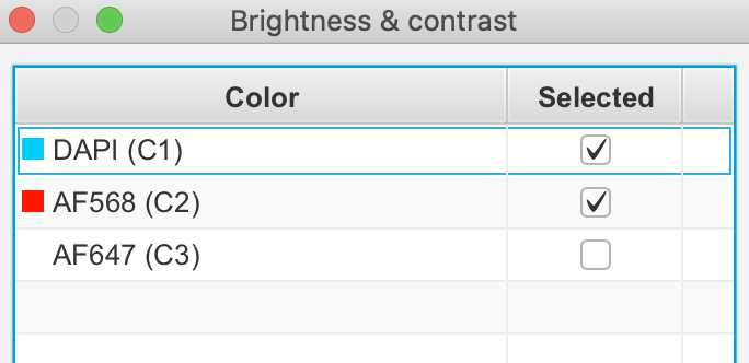
Double click on any channel to change its name and color.

Note: the original scan colors are not permanent and can be changed to make visualization easier. Note: the original scan colors are not permanent and can be changed to make visualization easier.

Tip: complementary colors (e.g. red and green, yellow and purple) will be easiest to distinguish for visualization. Tip: complementary colors (e.g. red and green, yellow and purple) will be easiest to distinguish for visualization.

#尊敬的用户，由于网络监管政策的限制，部分内容暂时无法在本网站直接浏览。我们已经为您准备了相关原始数据和链接，感谢您的理解与支持。
https://lh7-us.googleusercontent.com/_ny5ytECjQCoQ2jmLyygFKi_LWy3TVKsyH7qm7bWqjjxgEUszKr-gY0JWFSTzKja_LJZN51xV6Dxea4-vroUQQeR-CLuTQWmR3mIe2ls5U1vIeFglozTSIEZ1b47Q3EL8qdcdNPpD7DbsXknfrLysg

Adjust the brightness and contrast of the image by changing the min and max display values using the slider.

Note: The default gamma value is 1. Note: The default gamma value is 1.

Tip: Refer to IHC experiments (e.g. from The Human Protein Atlas) to help visualize expected stain localization and intensity. Tip: Refer to IHC experiments (e.g. from The Human Protein Atlas) to help visualize expected stain localization and intensity.

Use rectangle tool to select region of interest.

Rotate the rectangle by using the transform tool ( Objects: Annotations: Transform annotations ).

Select the rectangle and run the following script ( Automate: Show script editor ).

Note: if lengthwise sections are preferred, change "d1 < d2" to "d1 > d2" (on line 45 of the script). Note: if lengthwise sections are preferred, change "d1 < d2" to "d1 > d2" (on line 45 of the script).

_Tip: change the name for each region of interest by changing the ROI number ("ROI 1 Layer {i+1}") on the last line of the script.

-----------------------------------------------------------------------------------------------

/**
 * Split a rectangle into equal parts along its longest dimension.
 * Rotated rectangles are supported.
 * 
 * Written for https://forum.image.sc/t/how-to-divide-annotation-roi-into-equal-dimension-bins/51563/8
 *
 * @author Pete Bankhead
 * Taken from https://gist.github.com/petebankhead/e177b07784460a76d70f89347edd988d
 */

// Number of regions to create
int nRegions = 10

// Get selected object
def selected = getSelectedObject()
if (selected == null) {
    println 'No object selected!'
}

// Get points, removing duplicates
def roi = selected.getROI()
def points = new LinkedHashSet<>(roi.getAllPoints()) as List
if (points.size() != 4) {
    println 'I need a ROI with exactly 4 points'
    return
}

// Get the side lengths
double d1 = points[1].distance(points[0])
double d2 = points[2].distance(points[1])
double d3 = points[3].distance(points[2])
double d4 = points[0].distance(points[3])

// Check we really have a rectangle
// (Set this to a higher number of it's too strict)
double eps = 0.01
if (Math.abs(d1 - d3) > eps || Math.abs(d4 - d2) > eps) {
    println 'Points do not appear to form a rectangle!'
    return
}

// Get starting point based on longest side
int ind = 0
if (d1 < d2) {
    points.add(0, points.remove(3))
}
double x = points[ind].x
double y = points[ind].y
double dx = (points[ind+1].x - x) / nRegions
double dy = (points[ind+1].y - y) / nRegions
double dx2 = (points[ind+2].x - points[ind+1].x)
double dy2 = (points[ind+2].y - points[ind+1].y)

// Add annotations
def annotations = []
for (int i = 0; i < nRegions; i++) {
    double originX = x + dx*i
    double originY = y + dy*i
    def polygon = ROIs.createPolygonROI(
        [originX, originX+dx, originX+dx+dx2, originX+dx2] as double[],
        [originY, originY+dy, originY+dy+dy2, originY+dy2] as double[],
        roi.getImagePlane()
    )
    def newAnnotation = PathObjects.createAnnotationObject(polygon)
    newAnnotation.setName("ROI 1 Layer ${i+1}") //To change ROI number 
    annotations << newAnnotation
}

addObjects(annotations)
-----------------------------------------------------------------------------------------------

#尊敬的用户，由于网络监管政策的限制，部分内容暂时无法在本网站直接浏览。我们已经为您准备了相关原始数据和链接，感谢您的理解与支持。
https://lh7-us.googleusercontent.com/HNcBPwhLFVqh14Jb9mIde0WWISlDjEN4CswEa6BOSv6u5TxMsuWFPddBMhaSnOMTehC7Xyl2WsEl__WNovCh9OXglu6nbA2qOrnx6A4ut1v-r3F_T9OMpJinjhfSrjLcuN0KYvsvwiWJdyaV9c4b6A

Rename Annotations by right clicking on the selected layer then select Set properties .

#尊敬的用户，由于网络监管政策的限制，部分内容暂时无法在本网站直接浏览。我们已经为您准备了相关原始数据和链接，感谢您的理解与支持。
https://lh7-us.googleusercontent.com/9fIfnJ3X5US-WHbL7CGx8ZG8NQoLRXR8i7ub0Oc3J-5zyFDWXnRTGjMJqE_E6n2eQTL7OpL_KJh77q69Talam-LsBQTkN1VGmZ4qOrpxBaGBly8Uzm_nydWPWBS3cBvPcIL4BUMHb-Ty1R2UQdK1Yw

Select the region (largest rectangle) and click on Analyze: Cell detection: Positive Cell Detection .

Select the desired stain for cell detection by clicking on the drop down menu next to Detection channel .

Modify the Threshold value such that all positive cells are accounted for.

Note: a threshold of 300-400 would be ideal for a DAPI nuclei stain. Note: a threshold of 300-400 would be ideal for a DAPI nuclei stain.

Change the Score compartment by clicking on the dropdown menu next to it such that the stain selected matches its localization within the cell.

Note: it is easier to adjust the threshold when stain localization is known (e.g. Nucleus: DAPI max) Note: it is easier to adjust the threshold when stain localization is known (e.g. Nucleus: DAPI max)

Tip: if unsure about stain localization, select the cell option for easiest detection. Tip: if unsure about stain localization, select the cell option for easiest detection.

#尊敬的用户，由于网络监管政策的限制，部分内容暂时无法在本网站直接浏览。我们已经为您准备了相关原始数据和链接，感谢您的理解与支持。
https://lh7-us.googleusercontent.com/o8ONhX7Rk1Ddndnn-KCWzop5DrGPfAnaLQdQLnCPjX3d5dTjuEiZAW_VJoooO1VTVC4qe3P3f9RyxVK8zaado_ROEOfpjXNZ26dBRSOYoGDgvqKa3f2L3C-iHPOcqmc1UBvqXC_ZjGH0Ukqm3iDXvg

Click Run to start positive cell detection.

• Keep adjusting the Threshold value until the correct cells are detected.
• Note: it may take several adjustments to optimize the threshold value, zoom in and our of the image, if necessary, to help determine appropriate detection.
• Repeat for other regions

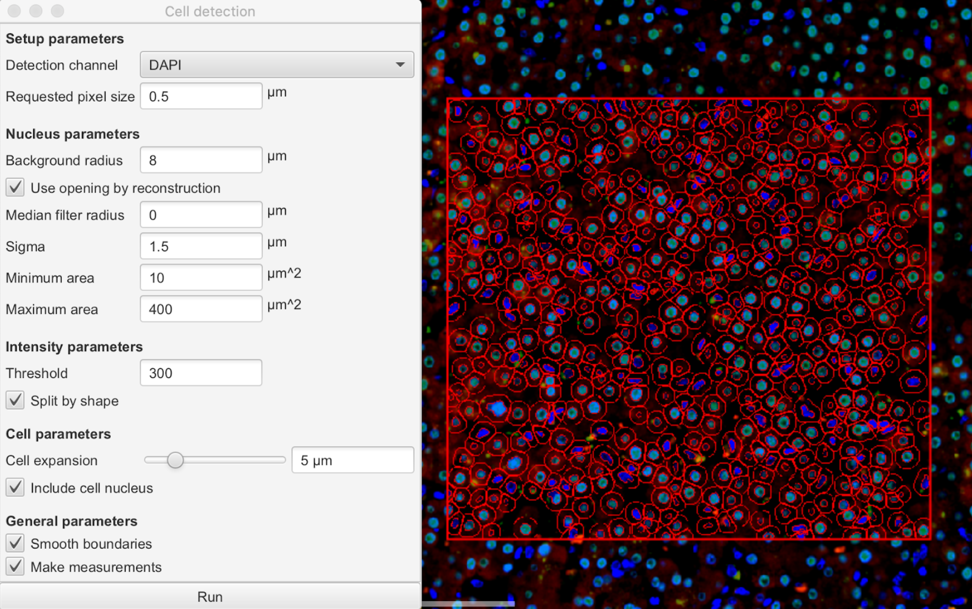
Select the annotation and run cell detection by clicking Analyze: Cell detection: Cell detection .

Select the desired stain for cell detection by clicking on the drop down menu next to Detection channel .

Modify the Threshold value such that all positive cells are accounted for.

Note: a threshold of 300-400 would be ideal for a DAPI nuclei stain. Note: a threshold of 300-400 would be ideal for a DAPI nuclei stain.

Change the Score compartment by clicking on the dropdown menu next to it such that the stain selected matches its localization within the cell.

Note: it is easier to adjust the threshold when stain localization is known (e.g. Nucleus: DAPI max) Note: it is easier to adjust the threshold when stain localization is known (e.g. Nucleus: DAPI max)

Tip: if unsure about stain localization, select the cell option for easiest detection. Tip: if unsure about stain localization, select the cell option for easiest detection.

If only cell detection or cell count is required, skip steps 12 to 16 and move forward with the file export. * If co-localization assessment is required proceed to step 12.

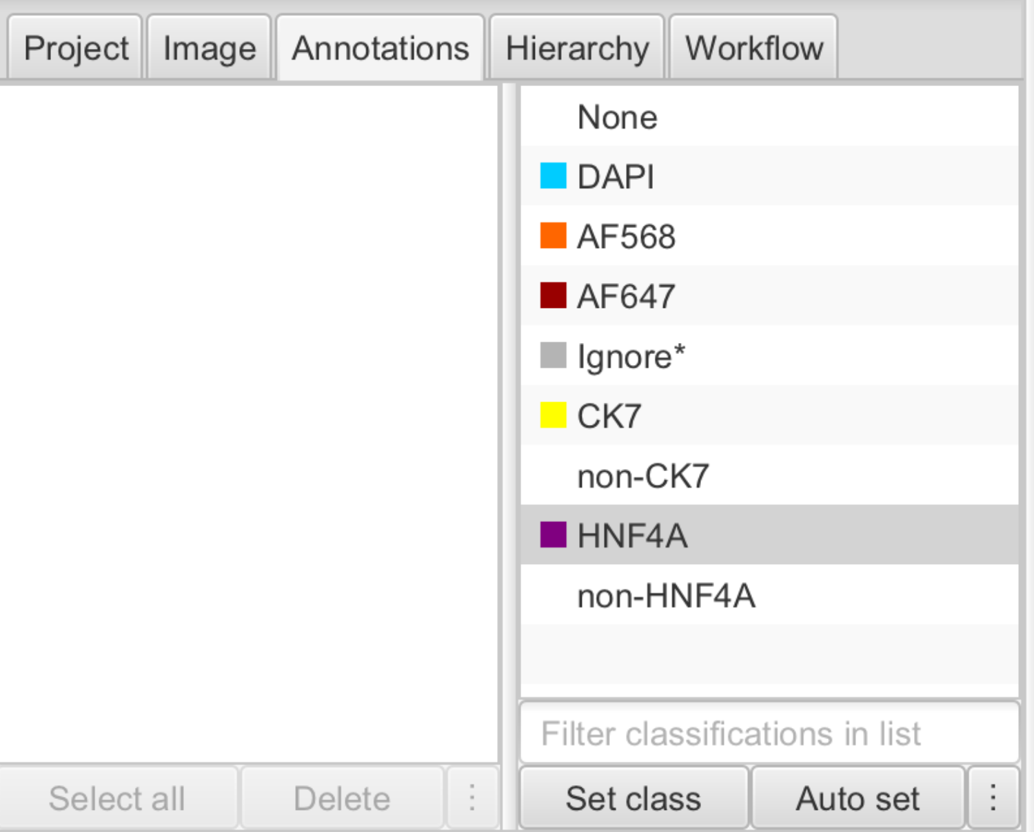
Create new classes by going to Annotations , and right clicking on the class list to add a new class.

Tip: Tip: creating classes for both positive and negative cells makes classification easier (e.g. HNF4A and non-HNF4A).

Create cell classifications by clicking Classify: Object classification: Create single measurement classifier .

Select the desired channel filter (e.g. DAPI, AF647) by clicking on the dropdown menu next to Object filter .

Adjust the Threshold using the slider.

Note: turn on live preview for better visualization. Note: turn on live preview for better visualization.

Save the classifier using the stain name.

#尊敬的用户，由于网络监管政策的限制，部分内容暂时无法在本网站直接浏览。我们已经为您准备了相关原始数据和链接，感谢您的理解与支持。
https://lh7-us.googleusercontent.com/fpztgIevmVFN95itXIY0HUPijU7dw2XtDV7IYcQc1qz4HZxb-OguaoaCoVfbKUGxQhj8gWghDmhCcK3AMn0nRgmk9tzcKclE22vyII9MmEcGn5usF8cuh9SZl8T_WSYhpanZ2Io1WI0Z63pvDTcHDw

Select the region of interest (previously selected using the rectangle tool).

Classify object by clicking Classify: Object classification: Load object classifier .

Apply object classification by clicking on the name of each classifier then clicking Apply classifier .

Tip: To apply more than one classifier to the same region select both using the command or control key and click Apply classifier sequentially. Tip: To apply more than one classifier to the same region select both using the command or control key and click Apply classifier sequentially .

#尊敬的用户，由于网络监管政策的限制，部分内容暂时无法在本网站直接浏览。我们已经为您准备了相关原始数据和链接，感谢您的理解与支持。
https://lh7-us.googleusercontent.com/RlL8u3p5M8avzY07HbUaH6J_jkEAOV3oxLigTDUrYJR67DCI767An4F9HsHMulqAmIBWDjOyz9eIfLdhaveQnKXnfWlJtANUe9TPuTCbJfGzxLqLinI6oxxXhy44zD2m9wgDs6Ds20geQtexS3KRmg

Click on Measurements: Export measurements to export data into a tsv file.

• Click on export annotations.
• Click on browse to select a name and file path for the export. Note: the generated tsv file can be opened on spreadsheet programs such as Microsoft Excel and copied to data analyzing softwares. Note: the generated tsv file can be opened on spreadsheet programs such as Microsoft Excel and copied to data analyzing softwares.