Protein Structural Modeling for Electron Microscopy Maps Using VESPER and MAINMAST
Eman Alnabati, Eman Alnabati, Genki Terashi, Genki Terashi, Daisuke Kihara, Daisuke Kihara
cryo-EM alignment
de novo protein modeling
electron microscopy maps
protein fitting
protein structure
Abstract
An increasing number of protein structures are determined by cryo-electron microscopy (cryo-EM) and stored in the Electron Microscopy Data Bank (EMDB). To interpret determined cryo-EM maps, several methods have been developed that model the tertiary structure of biomolecules, particularly proteins. Here we show how to use two such methods, VESPER and MAINMAST, which were developed in our group. VESPER is a method mainly for two purposes: fitting protein structure models into an EM map and aligning two EM maps locally or globally to capture their similarity. VESPER represents each EM map as a set of vectors pointing toward denser points. By considering matching the directions of vectors, in general, VESPER aligns maps better than conventional methods that only consider local densities of maps. MAINMAST is a de novo protein modeling tool designed for EM maps with resolution of 3–5 Å or better. MAINMAST builds a protein main chain directly from a density map by tracing dense points in an EM map and connecting them using a tree-graph structure. This article describes how to use these two tools using three illustrative modeling examples. © 2022 The Authors. Current Protocols published by Wiley Periodicals LLC.
Basic Protocol 1 : Protein structure model fitting using VESPER
Alternate Protocol : Atomic model fitting using VESPER web server
Basic Protocol 2 : Protein de novo modeling using MAINMAST
INTRODUCTION
Proteins are essential components of cells, performing a diverse range of biological functions. As the three-dimensional structure of proteins is crucial for understanding molecular mechanisms of their biological functions, structures have been determined by experimental methods including cryogenic-electron microscopy (cryo-EM). The number of maps determined by cryo-EM microscopy has increased rapidly due to the advances in direct detectors and image-processing algorithms (Nogales, 2016; Wu & Lander, 2020). The Electron Microscopy Data Bank (EMDB; Lawson et al., 2016) currently holds over 19,000 cryo-EM maps.
A variety of methods have been developed for structure modeling from cryo-EM maps (Alnabati & Kihara, 2019; Esquivel-Rodriguez & Kihara, 2013; Malhotra, Trager, Dal Peraro, & Topf, 2019). These methods could be roughly classified into three main categories according to map resolution. For high-resolution maps, de novo methods are designed to build protein main chains directly from density maps. Examples of de novo methods include tools provided in Phenix (Terwilliger, Adams, Afonine, & Sobolev, 2018), Rosetta (R. Y. Wang et al., 2015), MAINMAST (Terashi & Kihara, 2018a), and DeepTracer (Pfab, Phan, & Si, 2021). For intermediate-resolution maps (about 4–5 Å or worse), structures that were experimentally determined, or computational structure models (Jumper et al., 2021; Jain et al. (2021) could be fit to the density. Tools for fitting include iMODfit (Lopez-Blanco & Chacon, 2013), Flex-EM (Topf et al., 2008), IMP::BayesianEM (Bonomi et al., 2019), γ-Tempy (Pandurangan, Vasishtan, Alber, & Topf, 2015), and VESPER (Han, Terashi, Christoffer, Chen, & Kihara, 2021). At an intermediate resolution, one can also use deep learning–based tools, Emap2sec (Maddhuri Venkata Subramaniya, Terashi, & Kihara, 2019) and Emap2sec+ (X. Wang et al., 2021).
Here, we introduce how to use our methods, VESPER (Han et al., 2021) and MAINMAST (Terashi & Kihara, 2018a, 2018b; Terashi, Zha, & Kihara, 2020). Both methods are based on the importance of identifying local dense regions in cryo-EM maps, which are more likely to correspond to atoms of biomolecules in the map. VESPER aligns two EM maps, experimental maps, or simulated maps for a structure model, either locally or globally, by matching unit vectors that point toward dense points in maps. VESPER would be particularly useful for fitting computational models of protein structures into a map, which may be built by recent protein structure prediction methods (Christoffer, Bharadwaj, Luu, & Kihara, 2021; Jain et al., 2021; Tunyasuvunakool et al., 2021). MAINMAST builds a protein main chain directly from an EM map of resolution ∼4–5 Å or better by identifying dense points in the cryo-EM map, then connecting them by a tree data structure called a minimum spanning tree. After that, the amino acid sequence of the protein is mapped on the identified main-chain trace, which is a path in the tree structure. These two tools are provided as a part of cryo-EM software suites from our research group and are available at https://kiharalab.org/emsuites/.
Overview of the Software
Here we briefly explain the algorithms of VESPER and MAINMAST.
VESPER
VESPER (VEctor-based local SPace ElectRon density map alignment) is a computational tool for local and global alignment and comparison of cryo-EM maps (Han et al., 2021). VESPER represents a cryo-EM map as a set of vectors pointing toward denser density points, resulting in capturing local molecular structures in the map. The VESPER method aligns two EM maps in three main steps (Fig. 1). The first is converting each EM map to a set of unit vectors located at voxels with a density value larger than or equal to the author-recommended contour level (Fig. 1A and 1B). Unit vectors represent density points in the EM map, and they show the gradients of the density toward neighboring local high-density representative points. The next step is identifying the best alignments of the two maps by searching the reference map to allocate good poses of the target map (Fig. 1C). For each rotation in the set of sampled rotations using 30° or a user-defined interval, a translation scan is performed using Fast Fourier Transform (FFT), which speeds up the translation time (Frigo & Johnson, 2005), to optimize the sum of dot products of matched vectors from the two maps (DOT score). The position with the highest DOT score is added to the set of candidate superimpositions. The value of the dot product of two matched vectors ranges from −1 to 1, in which 1 indicates a perfect match, 0 means the matched vectors are perpendicular to each other, and −1 means the two vectors are pointing in opposite directions. Lastly, VESPER performs a finer rotational refinement of the best-scored search results (Fig. 1D). For each of the top 10 or user-specified number of superimposed models, VESPER performs a 5° local refinement along each axis if the rotational interval is larger than 5°, and writes the top refined models into the output file. To compare two alignments of two pairs of EM maps, using the raw DOT score is inconvenient because it has a dependency on the map size. Thus, we also compute the normalized Z-score of the DOT score. First, The DOT scores of the entire distribution of superimpositions are clustered, then the mean and the standard deviation of the largest cluster are computed. The Z-score score of each of the top models is then defined as (DOT score – mean)/standard deviation.
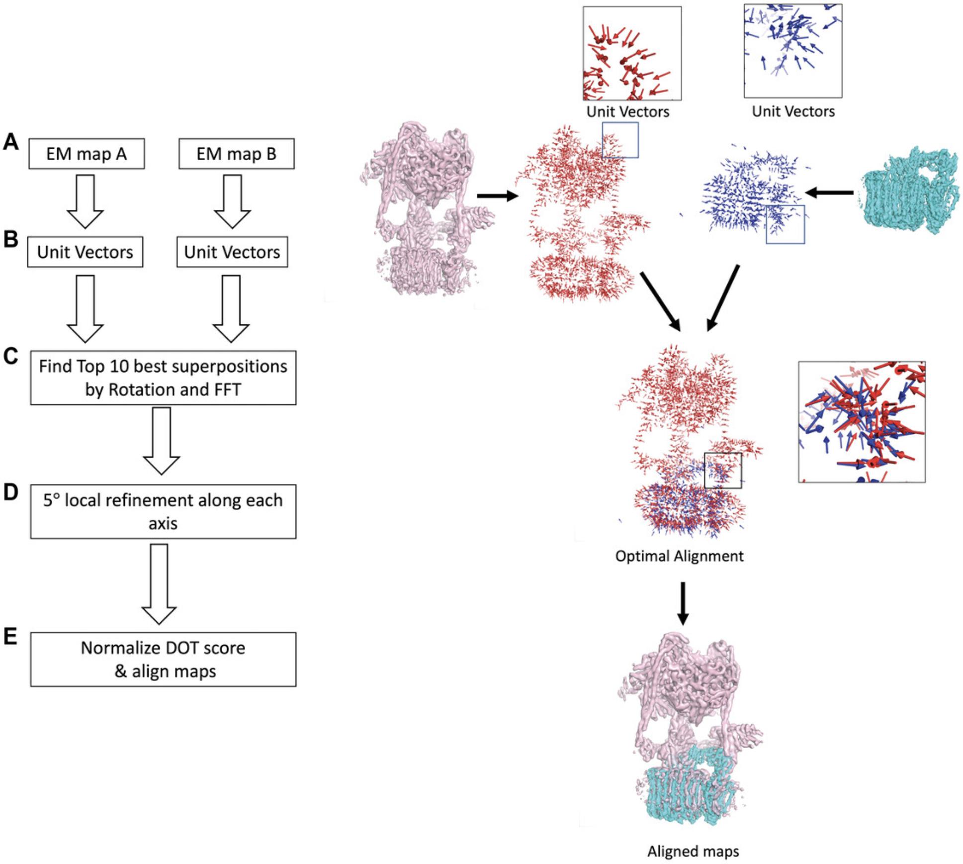
Aligning two cryo-EM maps using VESPER has several strengths. The first strength of VESPER is the scoring function, the DOT score, which leads to a better performance of VESPER over conventional methods that rely only on local densities of EM maps. In addition to its performance, the VESPER method is parallelized, allowing users to speed up the alignment process and handle large EM maps efficiently. Also, VESPER outputs ten alignments or a user-specified number of top alignments. Lastly, VESPER is also available as a web server, in which users can run VESPER without the need to download or install any files.
VESPER is available in two versions, as a program and as a web server. In the VESPER web server, users do not need to install any software, and they have the option to upload EM maps or specify their EMDB IDs. On the other hand, the VESPER program provides more options than the web server, which allows users to further customize the results.
MAINMAST
MAINMAST (MAINchain Model trAcing from Spanning Tree) is a fully automated de novo tool for building three-dimensional models of a protein main chain from a near-atomic-resolution EM map (Terashi & Kihara, 2018a; Terashi et al., 2020). MAINMAST traces local dense regions of the EM map, which tend to relate to protein main chain and side chains, and identifies Cα positions as tree-graph structures in the EM map. The MAINMAST algorithm consists of five main steps (Fig. 2). First, it identifies local dense points (LDPs) in a given EM map by the mean shift clustering algorithm (Carreira-Perpinan, 2006) using the assumption that dense regions in the EM map reflect the existence of atoms. The mean shift algorithm iteratively updates the locations of density points toward neighboring denser points and then clusters them until a small set of representative local dense points is obtained (see Commentary). After identifying LDPs, MAINMAST connects them using a minimum spanning tree (MST), which is a graph structure that connects all vertices without cycles and with minimum total edge weight. The weight of an edge is defined as the Euclidean distance between a pair of LDPs connected by that edge. Third, the MST is refined iteratively using a tabu search algorithm to find the protein main-chain path in the map. Usually, the longest path in the MST captures a large fraction of the correct main-chain trace, but with some incorrect connections or disconnections. Using different combinations of parameters, a pool of trees is generated and then ranked by a threading score which evaluates the alignment of the protein amino acid sequence to a path in a tree. The fourth step is identifying the longest path in MST and assigning protein amino acids to the local densities along that path. Finally, the full-atom model is generated from each Cα model using the PULCHRA program (Rotkiewicz & Skolnick, 2008) and refined using any refinement tools such as molecular dynamics flexible fitting (MDFF; McGreevy, Teo, Singharoy, & Schulten, 2016) or Rosetta relax (Nivon, Moretti, & Baker, 2013).
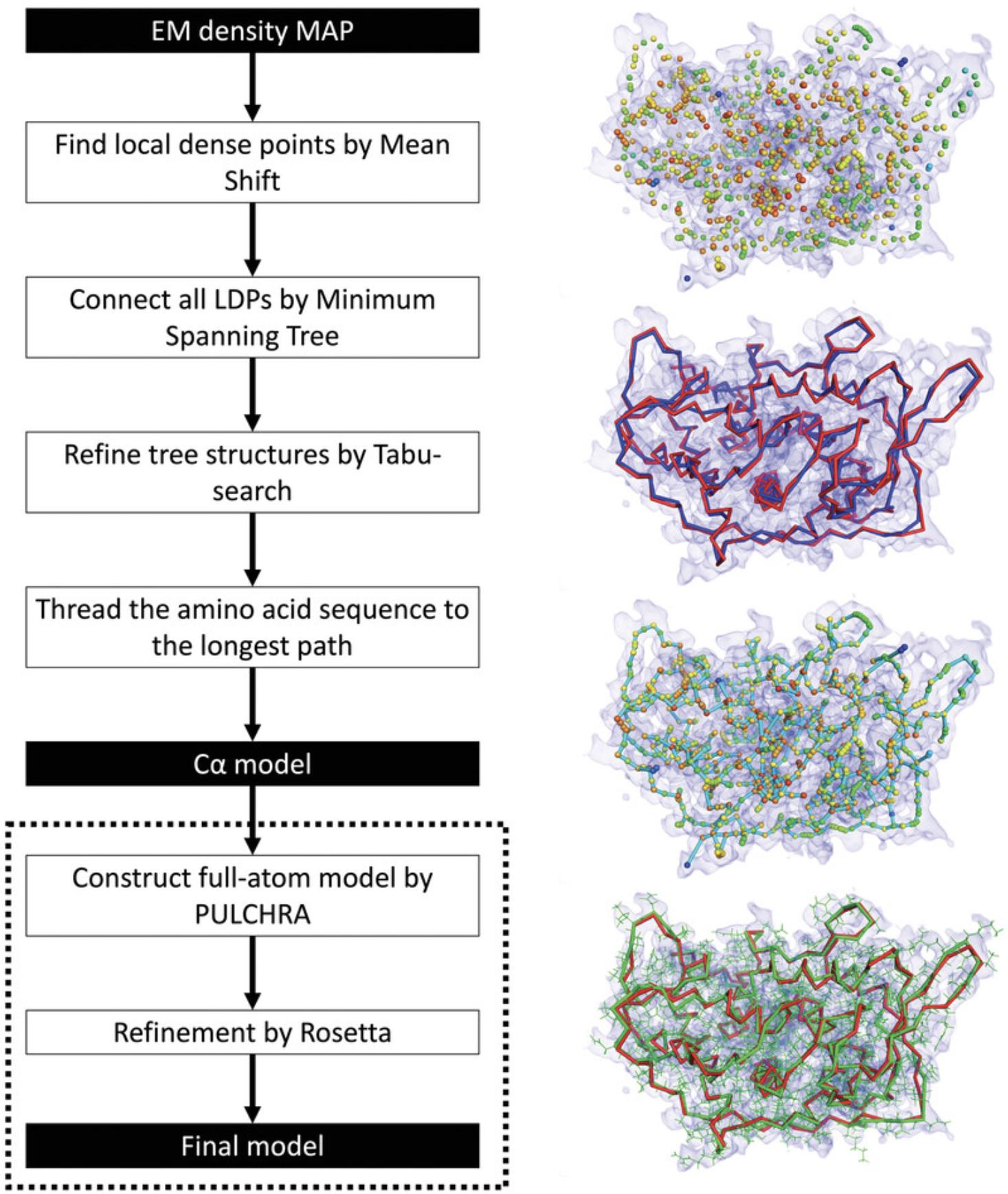
Building protein main chains from cryo-EM maps using MAINMAST has several advantages. First, MAINMAST builds protein structure models directly from EM maps without using any reference structures or fragments. The dependency on such structures may limit the method to those known structures and prevent it from handling new conformations. Also, MAINMAST is fully automated and does not require any manual configuration. Nevertheless, users can customize the different parameters of MAINMAST or use different parameter settings multiple times to obtain a pool of different models. Finally, MAINMAST outputs the results of its intermediate steps; thus, users can visualize the results and have a better understanding of the model.
Basic Protocol 1: PROTEIN STRUCTURE MODEL FITTING USING VESPER
This protocol provides guidance on using the VESPER program to align two experimentally determined cryo-EM maps or to fit an atomic structure either determined by an experimental method or modeled using a computational tool into a cryo-EM map. The input required for this protocol is the reference experimental cryo-EM map and either a simulated cryo-EM map of an atomic structure or an experimental EM map. Transformations of the top 10 or user-specified number of superimpositions along with transformed models are outputted.
Necessary Resources
Hardware
Any computer with Linux or macOS operating system, at least i5 processor, and 16 GB RAM
Software
- Python version 3.8.10 or higher (https://www.python.org/downloads/)
- Numpy version 1.21.0 or higher (https://numpy.org/install/)
- SciPy version 1.7.0 or higher (https://scipy.org/install/)
- FFTW version 3.3.10 (http://www.fftw.org/download.html)
- PyMOL version 2.4.1 or higher (optional), which is used for visualization, (https://pymol.org/2/)
- GCC compiler version 9.4.0 or higher (https://gcc.gnu.org/)
Files
Two cryo-EM maps in the format of MRC or CCP4
Install VESPER program
1.Download the VESPER code from the VESPER GitHub page by opening the command line window and type:
- git clone https://github.com/kiharalab/VESPER
2.In the command line window, change the working directory to the directory containing VESPER code as follows:
- cd /your_path_to_VESPER/VESPER_code/
3.Compile VESPER source code to generate an executable version of the code called VESPER, then move it to VESPER main directory:
- make
- cp VESPER ../
Run VESPER program
4.Prepare input files by downloading a cryo-EM map from EMDB (https://www.emdataresource.org/) and a protein structure from PDB (https://www.rcsb.org/).
5.Generate a simulated cryo-EM map from the atomic structure using the molmap function in Chimera (https://www.cgl.ucsf.edu/chimera/) as shown below, or using any other software.
Open Chimera and run the following commands on the Chimera command line:
1.open path_to_PDB_file/file_name.pdb (open PDB structure) 2.open path_to_EM_map_file/map_file.mrc (open the EM map to which the PDB structure is fitted into) 3.molmap #0 [map_resolution] onGrid #1 (generate a simulated map using the experimental map properties) 4.volume #2 save path_to_save_map/file_name.mrc (save the generated EM map)
6.Open the command-line window to run the VESPER command and specify the different parameters as follows:
VESPER -a [MAP1.mrc] -b [MAP2.mrc] (other parameters) > [VESPER_output_filename]
- -a: Path to the reference cryo-EM map
- -b: Path to the target cryo-EM map
- -t: Density threshold of the reference map, default = 0.00
- -T: Density threshold of the target map, default = 0.00
- -s: Sampling grid space for resampling the EM maps, default = 7.0 Å
- -A: Sampling angle interval for defining a set of rotations, i.e., 360 ÷ angle interval, default = 30°
- -c: Number of CPU cores used for running VESPER in parallel, default = 2
- -g: Bandwidth of the gaussian filter, default = 16.0, and sigma = 0.5 × (float number)
- -N: Refine top [int] models, default = 10
- -S: Show top models in PDB format, default = false
- -V: Vector product mode, default = true
- -L: Overlap mode, default = false
- -C: Cross-correlation coefficient mode, default = false
- -P: Pearson's correlation coefficient mode, default = false
- -F: Laplacian filtering mode, default = false
- -E: Evaluation mode of the current position, default = false
VESPER output is written to a file named VESPER_output_filename, which includes the top 10 or user-specified number of transformations applied on the target EM map to align it with the reference EM map, along with several scores evaluating the alignments. Also, the output file has the vector information of the top models. Each vector is represented by two atoms, Cα for the start position and Cβ for the end position.
VESPER -a emd_3342.map -b molmap_5fwm_transformed.mrc -t 0.015 -T 0.2 -s 3 -A 10 -c 20 -S true > vesper_result_3_10.txt
7.To transform a target density map according to the rotation and translation of each of the top alignments in VESPER output, run the following command:
python transform_em_map.py [parameters]
- -i1 or --input1: Name of the reference EM map file
- -i2 or --input2: Name of the target EM map file
- -t: Name of the result file from VESPER
- -odir (optional): Directory to store the generated transformed target EM map files. If not specified, the transformed target maps would be written to the current directory.
python transform_em_map.py -i1 emd_3342.map -i2 molmap_5fwm_transformed.mrc -t vesper_result_3_10.txt
The names of output files would have the following format: target_transform_model_#.mrc, in which # specifies the model number starting from 1.
Calculating normalized Z-score for top models in VESPER output file
8.To calculate the normalized Z-score of the top models in the VESPER output file, run the cluster_score.py script as follows:
python cluster_score.py -i [VESPER_output_filename] -c [Clustering cutoff] -o [Output_filename]
- -i: Name of the input file
- -c: Clustering cutoff for Z-scores which is used as follows: [Clustering cutoff × (Maximum DOT score – Minimum DOT score)] and it ranges from 0 to 1, default = 0.2
- -o: Output filename (optional): Name of the output file to store the normalized Z-scores of the models. If not specified, the output file would have the same name as the input filename followed by .normzscore
python cluster_score.py -i vesper_result_3_10.txt -o normalized_Z_score_emd3342.txt
The output file will contain the Z-score of each model in the input file, one line for each model as shown below:
Visualizing VESPER results
| Normalized z-score for top 10 models: | |
| #0 | 16.768505095477142 |
| #1 | 16.7211460976927 |
| #2 | 16.677474206555694 |
| #3 | 16.49780033833288 |
| #4 | 15.465432251303666 |
| #5 | 15.44975116092615 |
| #6 | 15.382853401143898 |
| #7 | 15.26661155761643 |
| #8 | 15.138023713287225 |
| #9 | 15.070875549608642 |
9.To visualize the reference EM map (Fig. 3A), open PyMOL and run the following commands on the PyMOL command line:
- bg_color white (this command changes the background color from black to white)
- set normalize_ccp4_maps, 0
- load xxxx.mrc (replace xxxx with the EM map file name)
- isosurface xxxx_isosurface, xxxx, reference_contour_level (replace reference_contour_level with the author-recommended contour level of the reference map in EMDB)
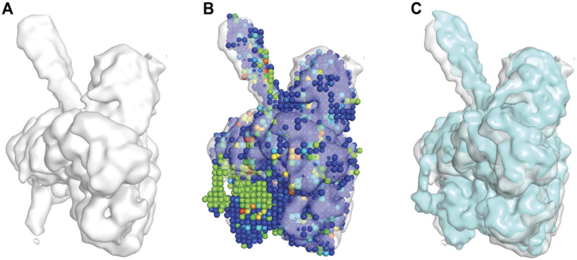
10.To visualize the PDB file containing vector representation of top models by VESPER (Fig. 3B), open PyMOL and run the following commands on the PyMOL command line:
- load xxxx.pdb, discrete =1 (replace xxxx by the file name you chose earlier in step 3)
- set transparency, 0.4
- hide cartoon, xxxx
- show spheres, xxxx
- spectrum b, rainbow_rev, xxxx
The PDB structures of top models will be shown as a set of spheres representing vectors, and spheres are colored based on their DOT score.
11.To visualize any of the MRC files of the top superimposed models generated in step 4 (Fig. 3C), open PyMOL and run the following commands in the PyMOL command line:
- load target_transform_model_#.mrc (Replace # with the model number you want to visualize)
- isosurface model#isosurface, target_transform_model#, target_contour_level (replace target_contour_level by the contour level used for the target map)
Alternate Protocol: ATOMIC MODEL FITTING USING VESPER WEB SERVER
This protocol provides guidance on using the VESPER web server for fitting an atomic model in a cryo-EM map or aligning two cryo-EM maps in a fast manner. Users can align two EM maps in a few steps without the need to download or install any files. Also, users can specify only a few parameter values while the rest of the parameters would have their default values. The Input required for this protocol is two cryo-EM maps or their EMDB IDs. An e-mail of the result files will be sent to the user after the computation is completed.
Necessary Resources
Hardware
Any up-to-date computer with internet access
Software
- An up-to-date web browser such as Google Chrome (https://www.google.com/chrome/) or Mozilla Firefox (https://www.mozilla.org/en-US/firefox/)
- PyMOL (optional), which is used for visualization (https://pymol.org/2/)
Files
- Besides using the search boxes to enter specific cryo-EM map IDs from EMDB, users can upload their cryo-EM maps. The density maps to be uploaded are in the format of MRC or CCP4.
Submit a job to the VESPER web server
1.Open the web browser and type the URL https://kiharalab.org/em-surfer/vesper.php. Figure 4 shows the VESPER web page, which contains a brief description of VESPER and how it works, three main boxes for specifying parameters, and the submit and reset buttons.
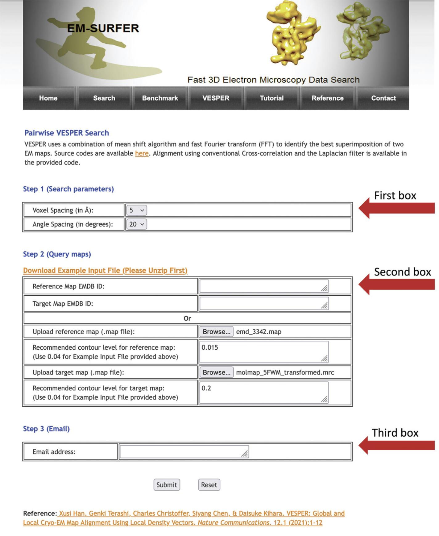
2.In the first box, Step 1 (Search parameters), specify voxel spacing in Angstroms to be applied on density maps. Three voxel spacing options are available, which are 5, 7, and 10 Å. The default voxel spacing is 7 Å. The second parameter to specify is the angular search degree. Choose one of the four angular search intervals, which are 20°, 30°, 60°, and 90° degrees.
3.The second box, Step 2 (Query maps), is for specifying cryo-EM maps and their density contour levels. You can either enter the EMDB ID of both reference and target maps or upload your density maps. For each map, specify the contour level to be used for that map.
4.In the last box, Step 3 (Email), enter a valid e-mail address, to which you want to receive VESPER results.
5.Once all parameters are entered, click on the submit button, which will show the following message: “Your request has been submitted! Once the result is ready, the result files will be sent to the e-mail specified.” After the computation is completed, you will receive an e-mail from sbit-admin@bio.purdue.edu titled “VESPER Calculation Result” with the results attached. The size of density maps along with voxel and angle intervals affect the amount of computation time needed. Small density maps will take a couple of minutes to be processed by VESPER.
6.The VESPER result e-mail will have a link to download archived result files, which include the following: an EM map of the reference structure, one PDB file that contains vectors in the target map, 10 MRC files for each of the top 10 models of the target EM map named target_transform_model_#.mrc, one text file contains normalized Z-scores of the top 10 alignments, and the VESPER_README.pdf file containing descriptions of result files and directions on how to visualize them.
Visualizing VESPER results
7.To visualize VESPER output files, follow steps 9, 10, and 11 of Basic Protocol 1.The only difference in the commands is in the file names. Use Reference.mrc for the reference map file in step 9 and customMapResult.pdb for the PDB file containing vector representation of top models in step 10.
Basic Protocol 2: PROTEIN DE NOVO MODELING USING MAINMAST
This protocol provides guidance on using MAINMAST for building a protein main chain directly from a cryo-EM map of resolution ∼4–5 Å or better. The required input files for this protocol are the reference cryo-EM map, protein chain sequence, and predicted secondary structure from protein sequence. The output is a Cα model of the protein main chain, from which a full-atom model could be constructed then refined.
Necessary Resources
Hardware
Any computer with Linux or macOS operating system, at least an i5 processor, and 16 GB RAM
Software
- Fortran version 9.4.0 or higher (https://fortran-lang.org/)
- Map2map procedure from SITUS package version 3.0 or higher (http://situs.biomachina.org/)
- SPIDER2 (https://github.com/yuedongyang/SPIDER2)
- PULCHRA version 3.04 or higher (https://www.pirx.com/pulchra/)
- PyMOL version 2.4.1 or higher (optional) for visualization: (https://pymol.org/2/)
Files
- Cryo-EM map of up to the size 150×150×150 (in the current setting, can be changed in the code)
- FASTA file which contains protein sequence
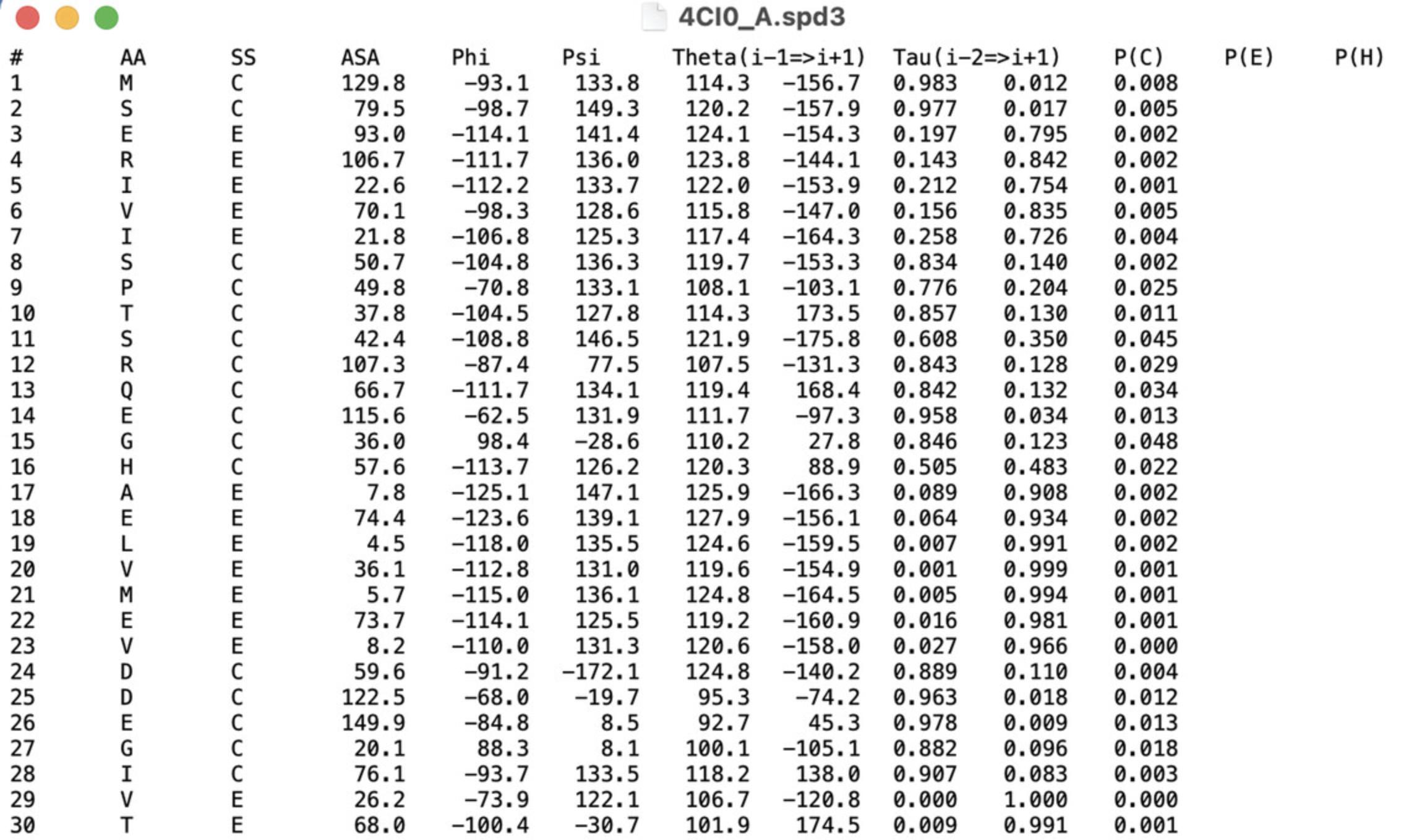
- SPD3 file which contains the secondary structure predicted by SPIDER2 (Fig. 5)
Install MAINMAST program
1.Download MAINMAST source code from https://kiharalab.org/mainmast/Downloads.html.
2.Open the command-line window and change the working directory to the directory containing the archived file. Then, unarchive MAINMAST.tgz by typing:
tar zxvf MAINMAST.tgz
- A new directory named MAINMAST/ will be generated.
3.Change the directory to MAINMAST by typing:
- cd MAINMAST
4.Compile the source code of the two main programs of MAINMAST by typing the following commands in the command-line command:
- gfortran MAINMAST.f -O3 -fbounds-check -o MAINMAST -mcmodel = medium
- gfortran ThreadCA.f -O3 -fbounds-check -o ThreadCA -mcmodel = medium
These commands will generate two executable programs, named MAINMAST and ThreadCA.
Run MAINMAST program
5.Prepare the following input files:
- a.If the density map is in MRC format, convert it to SITUS format by running the map2map procedure from SITUS packages as follows:
- echo 2|map2map density_map_name.mrc density_map_name.situs
- b.Predict protein secondary structures from protein amino acid sequence using SPIDER2 by running the following command:
- run_local.sh protein_seq_filename.seq
As an example, we used chain A of F420-reducing [NiFe] hydrogenase Frh, which has an EMD-2513 of resolution 3.36 Å and a fitted PDB structure with ID 4CI0. Chain A was manually segmented from the density map using Chimera's “zone tool.”
6.Run the first part of the MAINMAST program, which is called MAINMAST, to trace the protein main chain from the density map. The MAINMAST command identifies local dense points (LDPs) in the density map, which then are connected by a Minimum Spanning Tree (MST). After that, the MST is refined by a tabu search algorithm. The output is a PDB file representing each LDP in the longest path of the MST as a Cα atom.
- MAINMAST -m [density map file in situs format] (options) > path.pdb
Options in version 2.0:
- -Tree: Show MST mode
- -Graph: Show graph mode
Parameters for the mean shift clustering algorithm:
- -gw: Bandwidth of the gaussian filter; default = 2.0, sigma = 0.5 × [float]
- -Dkeep: Keep edge where distance < [float], default = 0.5
- -t: Threshold of density values, default = 0.0
- -allow: Max shift distance < [float], default = 10.0
- -filter: Filter of representative points, default = 0.1
- -merge: After the mean shift clustering, merge if distance < [float], default = 0.5
Parameters in Tabu-search:
- -Nround: Number of iterations, default = 5000
- -Nnb: Number of neighbors, default = 30
- -Ntb: Size of tabu-list, default = 100
- -Rlocal: Radius of Local MST, default = 10
- -Const: Constraint of total length of edge, default = 1.01, Total(Tree) < [float] × Total(MST)
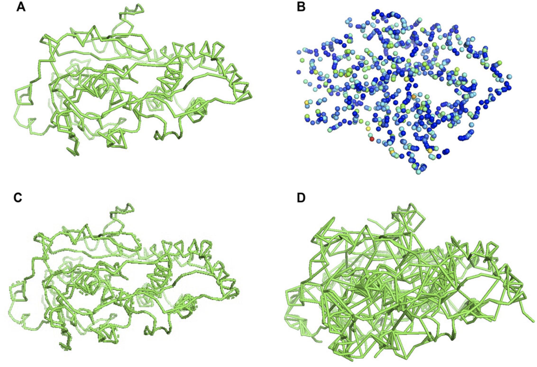
For our example, we used default parameter values except for density contour level and Dkeep, which determines the edge weight threshold used in the mean shift clustering algorithm, for which we used 0.045 (author-recommended contour level × 0.5), and 1.5, respectively. The output of the first part is shown in Figure 6A, which is a Cα model representing the LDPs on the longest path of the MST. This model is used as an input for the next step.
MAINMAST -i zoned_A.mrc -c 20 -t 0.045 -k 1.5 -R 10 > path.pdb
7.Run the second part of the MAINMAST program, which is called ThreadCA, to map the amino acid sequence on the longest path of the MST, as shown below. You can determine the direction of threading the protein amino acid sequence on the longest path in the refined tree graph from MAINMAST. The output of ThreadCA is a Cα model of the predicted protein chain.
- ThreadCA -i [output file from MAINMAST] -a [20AA.param] -spd [*.spd3] (options)
Options in version 1.0:
- -i: Result file of MAINMAST
- -a: 20AA.param
- -spd: Resulted file of SPIDER2
- -fw: Filter width, default = 1.0
- -Ab: Average length of CA-CA Bond, default = 3.5
- -Wb: Weight of Bond score, default = 0.9
- -r: Reverse mode, reverse protein main chain order
For chain A, we assigned the amino acid sequence in reverse order and used 1.3 and 3.4 for the parameters fw (filter width) and Ab (average length of C-C bonds), respectively. Default values were used for the other parameters. The output of ThreadCA, which is the Cα model of chain A is shown in Figure 7A.
ThreadCA -i path.pdb -a 20AA.param -spd 4CI0_A.spd3 -fw 1.3 -Ab 3.4 -Wb 0.9 -r >A_CA_reversed.pdb

8.Run PULCHRA on the output of ThreadCA, Cα model, to generate a full atom model. The full atom model can be then refined using any refinement methods such as Rosetta Relax (https://www.rosettacommons.org/) or MDFF (https://www.ks.uiuc.edu/Research/mdff/).
Visualizing MAINMAST results
9.To visualize a cryo-EM map, open PyMOL and run the following commands in the PyMOL command line:
- bg_color white
- set normalize_ccp4_maps, 0
- load xxxx (replace xxxx with map_file_name)
- isosurface xxxx_isosurface, emd_xxxx, reference_contour_level (replace reference_contour_level by the contour level used for the map)
10.To visualize the longest path of the MST generated by MAINMAST (Fig. 6A), run the bondmk.pl script, which takes as input the path PDB file generated in step 6 and outputs a PyMOL session file. Then, open the PyMOL session file of bondtree .pl using PyMOL:
- bondmk.pl path.pdb > path_session.txt
- pymol -u path_session.txt
11.To visualize the LDPs of the MST built in the density map (Fig. 6B):
-
Run MAINMAST in tree mode and save the output to thetree.pdbfile
-
Open PyMOL and run the following commands in the PyMOL command line:load tree.pdbset transparency, 0.4hide cartoon, treeshow spheres, treeset sphere_scale, 0.4, treespectrum b, selection = SEL, tree(color a molecule based on B-Factors)
12.To visualize the MST generated by MAINMAST using the tree mode (Fig. 6C) or to visualize all the possible connections, i.e., edges, on the EM map generated by MAINMAST using the graph mode (Fig. 6D), run the bondtree.pl script, which takes as input the output PDB file from MAINMAST and generates a PyMOL session file. Then, open the output file of bondtree.pl using PyMOL:
- bondtree.pl mainmast_output.pdb > pymol_session.txt
- pymol -u pymol_session.txt
GUIDELINES FOR UNDERSTANDING RESULTS
VESPER Results
VESPER outputs the best superimpositions of two cryo-EM maps according to their DOT score, which sums the dot product of their matched vectors. Other scores are also calculated for each of the superimposed models, which are overlap, cross-correlation, and Pearson's cross-correlation. The top models are sorted based on their DOT score, e.g., model 1 is the best-superimposed model that has the highest DOT score. Since the DOT score is dependent on map size, a normalized Z-score is provided. Details of the normalized Z-score calculations are in the “Overview of the Software” section. Empirically speaking, a normalized Z-score higher than 10.0 indicates a good alignment of the two density maps. Results of VESPER could vary depending on the combination of parameters that users choose. For voxel spacing and angle interval, resampling EM maps using 7 Å and rotating a target map using 30° along each axis showed a balance between alignment accuracy and computational speed. To improve alignment results, users could use smaller voxel and angle intervals, and to reduce computational time, users could use multiple CPU cores.
An Example of Atomic Fitting by VESPER
We showed an example of running both versions of VESPER on the structure of the Hsp90/Cdc37/Cdk4 complex (EMD-3342), which was determined at resolution 8 Å and a fitted PDB entry of 5FWM. To show the ability of VESPER to find the best fitting of PDB 5FWM in EMD-3342, we first randomly rotated and shifted the atomic structure, 5FWM. We ran the VESPER program using 3 Å and 10° for voxel spacing and angle interval, respectively. For the VESPER web server, we used 5 Å for voxel spacing and 20° for angle interval, as shown in Figure 4. Regarding density contour level, we used the author-recommended contour level for experimental map EMD-3342 and 0.2 for the simulated EM map of transformed PDB entry, 5FWM.
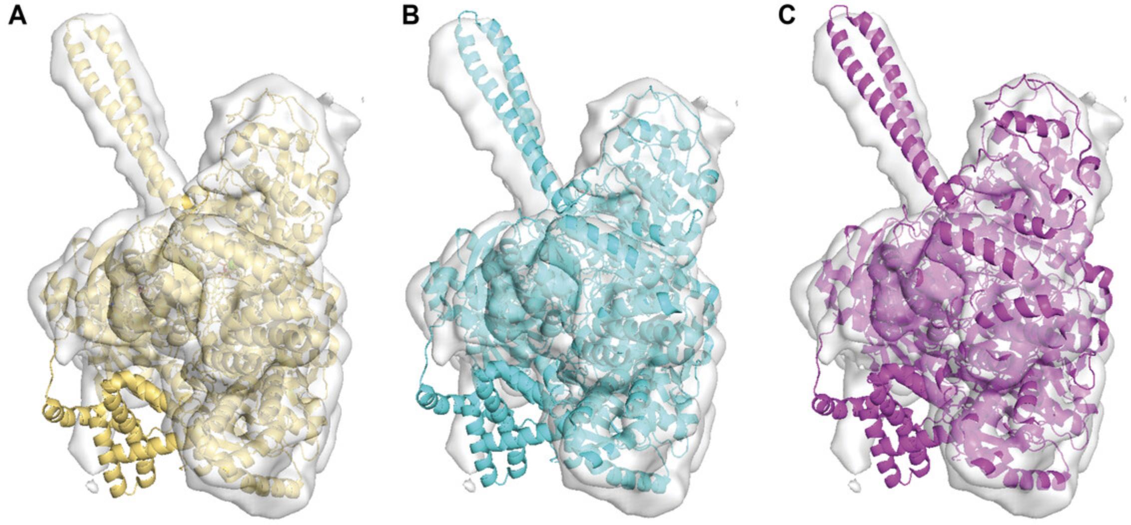
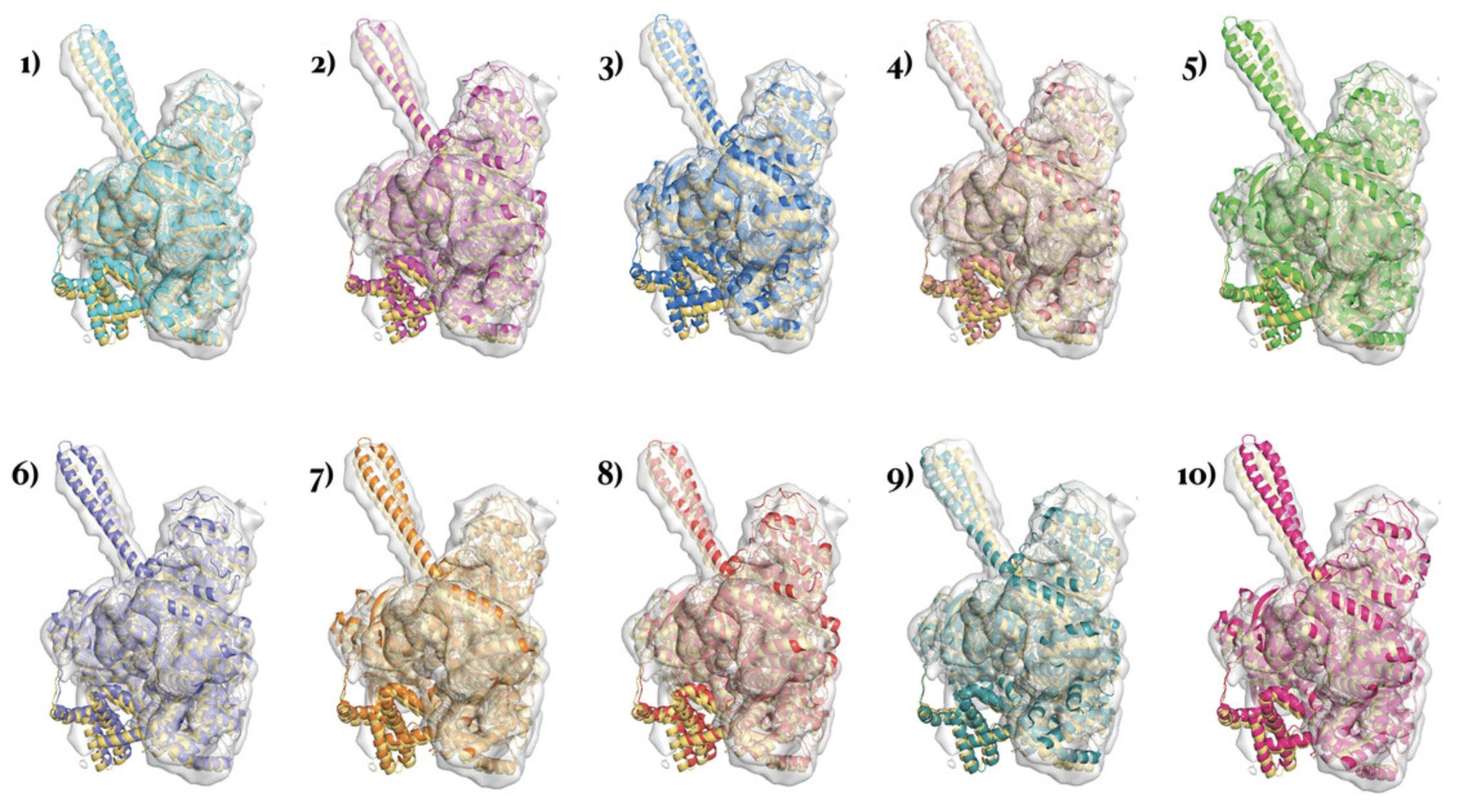
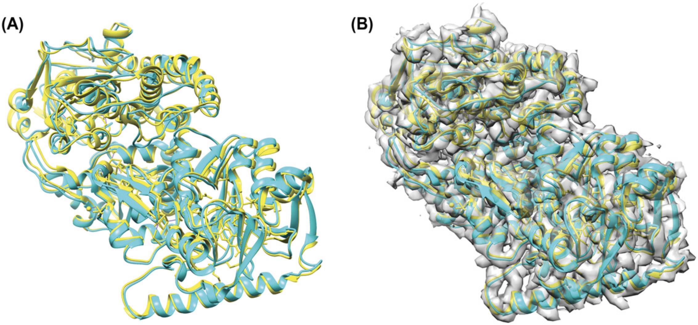
Both the VESPER program and the VESPER web server provided the top 10 models that have good alignment with the reference map, EMD-3342. Figure 8 shows the best-superimposed model identified by both versions of VESPER, where we can see a slightly better alignment in the best model of the VESPER program. To evaluate the result accuracy, we computed the root mean square deviation (RMSD) of top models and the reference structure, 5FWM. The RMSD values of top superimpositions of the VESPER program range from 3.44 to 4.93 Å, with an RMSD of 3.44 Å for the top 1 model. For the VESPER web server, the RMSD value of the top model is 5.8 Å and the RMSD values of the top 10 models range from 4.2 to 7.99 Å. The increase in RMSD values of the top 10 models of the VESPER server is due to the larger voxel and angle intervals used. The top 10 models of the VESPER program are shown in Figure 9. They have a good alignment with the reference structure, with small differences between them.
MAINMAST Results
MAINMAST builds a protein model from an EM map of a near-atomic resolution of around 4–5 Å or better by tracing local dense regions of the map. The MAINMAST program has two subprograms—MAINMAST and ThreadCA—and each of them outputs a Cα model. In the first Cα model, Cα atoms represent LDPs in the longest path of the MST, which represent the protein main chain. The second Cα model represents the protein main chain after threading the protein amino acid sequence on the MST's longest path. Users have the option to choose the direction of threading of the protein amino acid sequence on the longest path of MST. The protein full-atom model is then built from the Cα model using PULTCHRA software and refined using any refinement method. MAINMAST could be used with several parameter settings that result in a pool of models, users can choose from.
An Example of Protein Structure Building by MAINMAST
We showed an example of MAINMAST on chain A of F420-reducing [NiFe] hydrogenase Frh, which has EMD-2513 of resolution 3.36 Å and a fitted PDB structure with ID 4CI0. Chain A was manually segmented from the density map using Chimera's “zone tool.” Then, we ran the first part of MAINMAST using default parameter values except for density contour level and Dkeep, for which we used 0.045 (author-recommended contour level × 0.5) and 1.5, respectively. The output of the first part is shown in Figure 6A, which is a Cα model of the LDPs on the longest path of the MST. This Cα model is used as an input for the second part of MAINMAST, which is ThreadCA. Here we assigned the amino acid sequence in reverse order and used 1.3 and 3.4 for the parameters fw (filter width) and Ab (average length of Cα-Cα bonds), respectively. Default values were used for the other parameters. The output of ThreadCA, which is the Cα model of chain A is shown in Figure 7A.
To evaluate the resulted protein Cα model, we used the same metrics from the MAINMAST paper. These evaluation metrics are Cα RMSD, coverage, and precision. Cα RMSD is RMSD computed between only Cα atoms of the model relative to the corresponding Cα atoms of the reference structure. Coverage measures the fraction of Cα atoms in the reference structure that are within a certain distance cutoff (we used 3.0 Å) to any Cα atoms in the model. Precision computes the fraction of Cα atoms in the model that are within a 3.0 Å distance cutoff to any Cα atoms in the reference structure. The Cα RMSD, coverage, and precision values of the MAINMAST protein Cα model are 3.18 Å, 0.974, and 1, respectively. After that, the full-atom model of chain A was generated using PULCHRA and refined by Rosetta Relax (Fig. 7B). The refined model of chain A has an RMSD of 3.2 Å, coverage of 0.961, and precision of 0.997.
An Example of Combining VESPER and MAINMAST for Building a Protein Complex Structure
VESPER and MAINMAST aim to identify the structure of proteins from cryo-EM maps either by fitting their atomic structure into the EM map using VESPER or by building the protein model from the map density using MAINMAST. For an EM map of a protein complex where the atomic structure of some of its subunits is known but missing for the other subunits, we can combine the results of VESPER and MAINMAST to build the atomic structure of the entire protein complex. For demonstration, we used the same example that we used for MAINMAST in the previous section. PDB structure 4CI0 has three protein chains, A, B, and C. We assumed that the atomic structure of chain A was missing and built it using MAINMAST, as shown in “An Example of Protein Structure Building by MAINMAST,” above. For chains B and C, we used VESPER to fit their atomic structure in the EM map EMD-2513 after applying random shifting and rotation on them to change their initial position. Since all three protein chains fit a small region of EMD-2513, we segmented the overlapping region using Chimera's “zone tool” and used it as our reference density map for VESPER. When running VESPER, we used EMD-2513 voxel spacing, 10, and 0.6 for voxel interval, rotational interval, and density contour level of the simulated map of chains B and C, respectively. The best model of chains B and C has an RMSD of 2.12 Å, while the top 10 models’ RMSD values range from 2.07 to 2.75 Å. To generate the atomic model of PDB structure 4CI0, we combined the atomic model of chain A generated by MAINMAST and the top one atomic model of chains B and C from VESPER, as shown in Figure 10. The RMSD of the protein complex model is 2.64 Å.
COMMENTARY
Mean shift algorithm
MAINMAST uses the mean shift algorithm (Carreira-Perpinan, 2006), which is a non-parametric clustering method, for choosing representative local dense points (LDPs) in an EM map. LDPs usually correspond to atom positions in the map.
For an EM map with grid points
where σ is a bandwidth set to 1.0. After updating seed point positions, the density values of points
Then, the density is normalized as follows (see Equation 4): \begin{equation} {\rm{\Theta }}\left( y \right) = {\rm{;}}\frac{{{\rm{\Theta }}\left( y \right) - {{\rm{\Theta }}{min}}}}{{{{\rm{\Theta }}{max}} - {{\rm{\Theta }}_{min}}}} \end{equation}
where
Critical Parameters
In VESPER, several parameters affect EM map alignment accuracy. The first parameter is the voxel spacing used to resample the EM map. Since the search is based on the DOT score, which computes the alignment of unit vectors placed at map grids, changing the voxel spacing affects the DOT score, which changes the results drastically. Using small voxel spacing increases the number of grids and improves capturing the local characteristics of the map, while a large voxel spacing may miss some of these details. In addition to voxel spacing, angle interval plays an important role in density map alignment. A small angle interval allows for a more extensive search of the rotational space, which could lead to a better alignment. However, a small angle interval increases the computational time. The last important parameter in VESPER is the density contour level used to construct the isosurface shape of the density map. Density voxels with a density value higher than the density contour level have unit vectors assigned to them. Changing the density contour level affects the number of unit vectors, and therefore the DOT score.
In MAINMAST, several parameters could be critical in the protein modeling process. Running MAINMAST using different parameter settings allows users to customize and tune the results based on their map characteristics. The first important parameter is the density threshold used in constructing the shape of EM maps. For experimental EM maps, users could use (1, 0.5, or 0.25) × author-recommended contour level. Lowering an EM map contour level adds more voxels, to which a protein main chain could be assigned. Another important parameter is the sphere radius of local MSTs (Rlocal), which is used when connecting LDPs to construct the MST. Increasing the radius of local MSTs increases the size of local MSTs. Some of the possible values to use for this parameter are 5.0, 7.5, and 10.0 Å. The last parameter is the edge weight threshold (Dkeep) used when refining the initial MST using tabu search. The edge weight threshold prevents picking edges in the MST refinement process which leads to small changes. Some values that have been used in the MAINMAST datasets for this parameter are 0.5, 1.0, and 1.5 Å.
Troubleshooting
In Table 1, we listed a few common questions and problems when using the two software.
| Problem | Possible cause | Solution |
|---|---|---|
| Bad alignment results using VESPER | Wrong contour level for simulated EM map | Visualize the simulated EM map along with its fitted PDB structure. Choose a contour level that covers the entire PDB structure. |
| VESPER takes a very long time to align EM maps | VESPER slowness could be caused by using a very small voxel interval or rotational interval along with large EM maps | Increase voxel interval or rotational interval or both. Also, you could run VESPER using multiple CPU cores to reduce computational time. |
| Users cannot compile MAINMAST source code on macOS machines | Gfortran is not installed in the machine |
To compile MAINMAST source code, install Xcode, Homebrew, and gfortran as follows: 1. Download Xcode (https://developer.apple.com/xcode/). 2- Open the terminal from Applications and type: xcode-select --install /usr/bin/ruby -e "$(curl -fsSL https://raw.githubusercontent.com/Homebrew/install/master/install)" brew install gcc |
| Unable to run ThreadCA program when using MAINMAST | Missing one of the three input files: the output file from MAINMAST, the 20AA.param file, or the SPD3 file | First, run MAINMAST and use its output for ThreadCA along with the protein predicted secondary structure (SPD3 file) and the 20AA.param file provided with the MAINMAST code. |
| Receiving the following error when running MAINMAST: "Fortran runtime error: Index '301' of dimension 2 of array 'dmap' above upper bound of 300" | This error is caused by memory limitation in the MAINMAST program. MAINMAST handles an EM map of size 150×150×150 or smaller |
Reduce the size of the EM map: 1. By using the relion_image_handler command from the relion program, which shifts the map to its center-of-mass then changes its size to 100×100×100 as follows: relion_image_handler --i INPUT.mrc --new_box 100 - o OUTPUT.mrc - shift_com true 2. If a reference PDB structure is available, then use Chimera's “zone tool” to extract the region of the EM map which is within a specific distance of a set of atoms. |
| MAINMAST takes a very long time or provides models which look strange | Wrong density threshold is applied to the EM map. If the density threshold is low, then more density is considered, resulting in a longer computational time. On the other hand, if the density threshold is high, then MAINMAST does not have enough density to build models. |
Use author-recommended contour level of experimental EM maps if protein main chain is observed. If not, try (0.9, 0.8, …) × recommended contour level. Another way to decide the appropriate density threshold is by generating the MST by MAINMAST and checking if it covers the entire EM map or just a part of it, suggesting that the applied threshold is high. |
Acknowledgments
This work is partially supported by the National Institutes of Health (R01GM133840, R01GM123055, and 3R01GM133840-02S1) and the National Science Foundation (DBI2003635, DBI2146026, CMMI1825941, and MCB1925643). EA is supported by a fellowship from Umm Al-Qura University, Saudi Arabia.
Author Contributions
Eman Alnabati : data curation, formal analysis, investigation, writing original draft; Genki Terashi : methodology, software, supervision, validation, writing review and editing; Daisuke Kihara : conceptualization, data curation, funding acquisition, project administration, resources, supervision, validation, writing review and editing.
Conflict of Interest
The authors declare no competing interests.
Open Research
Data Availability Statement
The data that support the protocols are available at https://doi.org/10.5281/zenodo.6363352.
Literature Cited
- Alnabati, E., & Kihara, D. (2019). Advances in structure modeling methods for cryo-electron microscopy maps. Molecules (Basel, Switzerland) , 25(1), 82. doi: 10.3390/molecules25010082
- Bonomi, M., Hanot, S., Greenberg, C. H., Sali, A., Nilges, M., Vendruscolo, M., & Pellarin, R. (2019). Bayesian weighing of electron cryo-microscopy data for integrative structural modeling. Structure (London, England) , 27(1), 175–188.e176. doi: 10.1016/j.str.2018.09.011
- Carreira-Perpinan, M. A. (2006). Acceleration strategies for gaussian mean-shift image segmentation. IEEE Conference on Computer Vision and Pattern Recognition , 1, 1160–1167.
- Christoffer, C., Bharadwaj, V., Luu, R., & Kihara, D. (2021). LZerD Protein-Protein docking webserver enhanced with de novo structure prediction. Frontiers in Molecular Biosciences , 8, 724947. doi: 10.3389/fmolb.2021.724947
- Esquivel-Rodriguez, J., & Kihara, D. (2013). Computational methods for constructing protein structure models from 3D electron microscopy maps. Journal of Structural Biology , 184(1), 93–102. doi: 10.1016/j.jsb.2013.06.008
- Frigo, M., & Johnson, S. G. (2005). The design and implementation of FFTW3. Proceedings of the IEEE , 93, 216–231.
- Han, X., Terashi, G., Christoffer, C., Chen, S., & Kihara, D. (2021). VESPER: Global and local cryo-EM map alignment using local density vectors. Nature Communication , 12(1), 2090. doi: 10.1038/s41467-021-22401-y
- Jain, A., Terashi, G., Kagaya, Y., Maddhuri Venkata Subramaniya, S. R., Christoffer, C., & Kihara, D. (2021). Analyzing effect of quadruple multiple sequence alignments on deep learning based protein inter-residue distance prediction. Science Reports , 11(1), 7574. doi: 10.1038/s41598-021-87204-z
- Jumper, J., Evans, R., Pritzel, A., Green, T., Figurnov, M., Ronneberger, O., … Hassabis, D. (2021). Highly accurate protein structure prediction with AlphaFold. Nature , 596(7873), 583–589. doi: 10.1038/s41586-021-03819-2
- Lawson, C. L., Patwardhan, A., Baker, M. L., Hryc, C., Garcia, E. S., Hudson, B. P., … Chiu, W. (2016). EMDataBank unified data resource for 3DEM. Nucleic Acids Research , 44(D1), D396–403. doi: 10.1093/nar/gkv1126
- Lopez-Blanco, J. R., & Chacon, P. (2013). iMODFIT: Efficient and robust flexible fitting based on vibrational analysis in internal coordinates. Journal of Structural Biology , 184(2), 261–270. doi: 10.1016/j.jsb.2013.08.010
- Maddhuri Venkata Subramaniya, S. R., Terashi, G., & Kihara, D. (2019). Protein secondary structure detection in intermediate-resolution cryo-EM maps using deep learning. Nature Methods , 16(9), 911–917. doi: 10.1038/s41592-019-0500-1
- Malhotra, S., Trager, S., Dal Peraro, M., & Topf, M. (2019). Modelling structures in cryo-EM maps. Current Opinion in Structural Biology , 58, 105–114. doi: 10.1016/j.sbi.2019.05.024
- McGreevy, R., Teo, I., Singharoy, A., & Schulten, K. (2016). Advances in the molecular dynamics flexible fitting method for cryo-EM modeling. Methods (San Diego, Calif.) , 100, 50–60. doi: 10.1016/j.ymeth.2016.01.009
- Nivon, L. G., Moretti, R., & Baker, D. (2013). A Pareto-optimal refinement method for protein design scaffolds. Plos One , 8(4), e59004. doi: 10.1371/journal.pone.0059004
- Nogales, E. (2016). The development of cryo-EM into a mainstream structural biology technique. Nature Methods , 13, 24–27.
- Pandurangan, A. P., Vasishtan, D., Alber, F., & Topf, M. (2015). gamma-TEMPy: Simultaneous fitting of components in 3D-EM maps of their assembly using a genetic algorithm. Structure (London, England) , 23(12), 2365–2376. doi: 10.1016/j.str.2015.10.013
- Pfab, J., Phan, N. M., & Si, D. (2021). DeepTracer for fast de novo cryo-EM protein structure modeling and special studies on CoV-related complexes. Proceedings of the National Academy of Sciences of the United States of America , 118(2), e2017525118. doi: 10.1073/pnas.2017525118
- Rotkiewicz, P., & Skolnick, J. (2008). Fast procedure for reconstruction of full-atom protein models from reduced representations. Journal of Computational Chemistry , 29(9), 1460–1465. doi: 10.1002/jcc.20906
- Terashi, G., & Kihara, D. (2018a). De novo main-chain modeling for EM maps using MAINMAST. Nature Communication , 9(1), 1618. doi: 10.1038/s41467-018-04053-7
- Terashi, G., & Kihara, D. (2018b). De novo main-chain modeling with MAINMAST in 2015/2016 EM Model Challenge. Journal of Structural Biology , 204(2), 351–359. doi: 10.1016/j.jsb.2018.07.013
- Terashi, G., Zha, Y., & Kihara, D. (2020). Protein structure modeling from Cryo-EM map using MAINMAST and MAINMAST-GUI plugin. Methods in Molecular Biology , 2165, 317–336. doi: 10.1007/978-1-0716-0708-4_19
- Terwilliger, T. C., Adams, P. D., Afonine, P. V., & Sobolev, O. V. (2018). A fully automatic method yielding initial models from high-resolution cryo-electron microscopy maps. Nature Methods , 15(11), 905–908. doi: 10.1038/s41592-018-0173-1
- Topf, M., Lasker, K., Webb, B., Wolfson, H., Chiu, W., & Sali, A. (2008). Protein structure fitting and refinement guided by cryo-EM density. Structure (London, England) , 16(2), 295–307. doi: 10.1016/j.str.2007.11.016
- Tunyasuvunakool, K., Adler, J., Wu, Z., Green, T., Zielinski, M., Zidek, A., … Hassabis, D. (2021). Highly accurate protein structure prediction for the human proteome. Nature , 596(7873), 590–596. doi: 10.1038/s41586-021-03828-1
- Wang, R. Y., Kudryashev, M., Li, X., Egelman, E. H., Basler, M., Cheng, Y., … DiMaio, F. (2015). De novo protein structure determination from near-atomic-resolution cryo-EM maps. Nature Methods , 12(4), 335–338. doi: 10.1038/nmeth.3287
- Wang, X., Alnabati, E., Aderinwale, T. W., Maddhuri Venkata Subramaniya, S. R., Terashi, G., & Kihara, D. (2021). Detecting protein and DNA/RNA structures in cryo-EM maps of intermediate resolution using deep learning. Nature Communication , 12(1), 2302. doi: 10.1038/s41467-021-22577-3
- Wu, M., & Lander, G. C. (2020). Present and Emerging Methodologies in Cryo-EM Single-Particle Analysis. Biophysical Journal , 119(7), 1281–1289. doi: 10.1016/j.bpj.2020.08.027
Citing Literature
Number of times cited according to CrossRef: 4
- Nabin Giri, Liguo Wang, Jianlin Cheng, Cryo2StructData: A Large Labeled Cryo-EM Density Map Dataset for AI-based Modeling of Protein Structures, Scientific Data, 10.1038/s41597-024-03299-9, 11 , 1, (2024).
- Zhenjiao Du, Jeffrey Comer, Yonghui Li, Bioinformatics approaches to discovering food-derived bioactive peptides: Reviews and perspectives, TrAC Trends in Analytical Chemistry, 10.1016/j.trac.2023.117051, 162 , (117051), (2023).
- Nabin Giri, Raj S. Roy, Jianlin Cheng, Deep learning for reconstructing protein structures from cryo-EM density maps: Recent advances and future directions, Current Opinion in Structural Biology, 10.1016/j.sbi.2023.102536, 79 , (102536), (2023).
- Charles Christoffer, Daisuke Kihara, Domain-Based Protein Docking with Extremely Large Conformational Changes, Journal of Molecular Biology, 10.1016/j.jmb.2022.167820, 434 , 21, (167820), (2022).

