Using high-resolution microscopy data to generate realistic structures for electromagnetic FDTD simulations from complex biological models

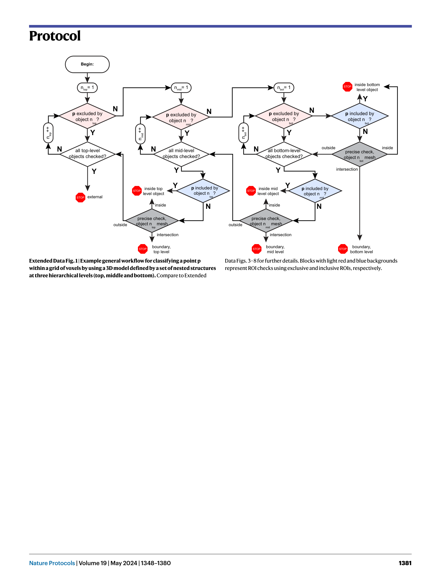
Extended Data Fig. 1 Example general workflow for classifying a point p within a grid of voxels by using a 3D model defined by a set of nested structures at three hierarchical levels (top, middle and bottom).

Compare to Extended Data Figs. 3 – 8 for further details. Blocks with light red and blue backgrounds represent ROI checks using exclusive and inclusive ROIs, respectively.

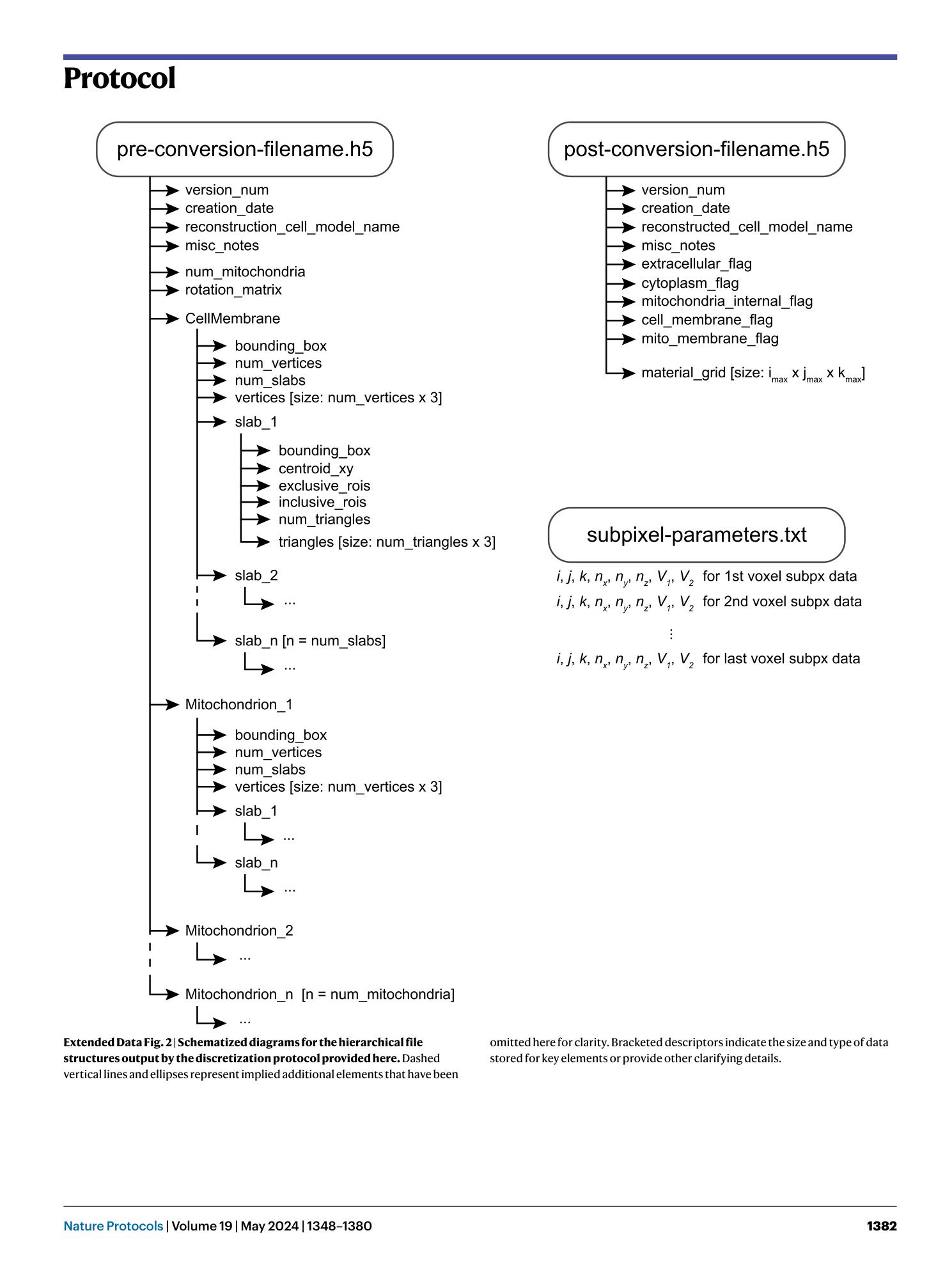
Extended Data Fig. 2 Schematized diagrams for the hierarchical file structures output by the discretization protocol provided here.

Dashed vertical lines and ellipses represent implied additional elements that have been omitted here for clarity. Bracketed descriptors indicate the size and type of data stored for key elements or provide other clarifying details.

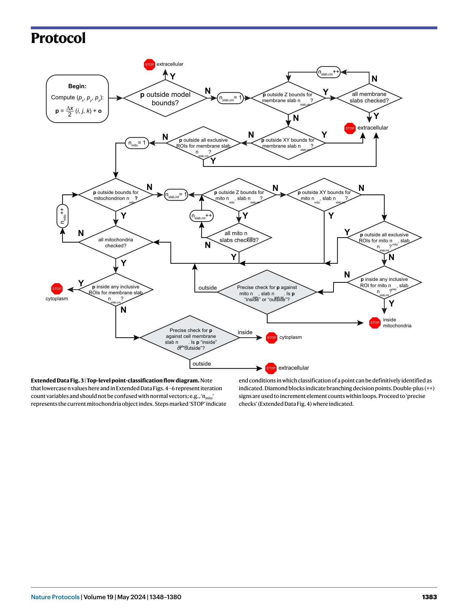
Extended Data Fig. 3 Top-level point-classification flow diagram.

Note that lowercase n values here and in Extended Data Figs. 4 – 6 represent iteration count variables and should not be confused with normal vectors; e.g., ‘n mito ’ represents the current mitochondria object index. Steps marked ‘STOP’ indicate end conditions in which classification of a point can be definitively identified as indicated. Diamond blocks indicate branching decision points. Double-plus (++) signs are used to increment element counts within loops. Proceed to ‘precise checks’ (Extended Data Fig. 4 ) where indicated.

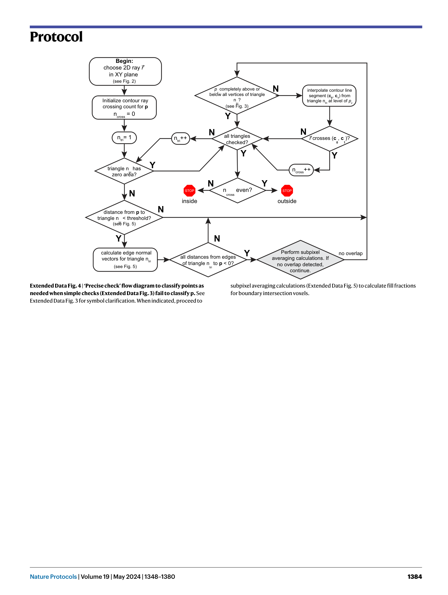
[ Extended Data Fig. 4 ‘Precise check’ flow diagram to classify points as needed when simple checks (Extended Data Fig. 3 ) fail to classify p . ](https://www.nature.com/articles/s41596-023-00947-z/figures/13)

See Extended Data Fig. 3 for symbol clarification. When indicated, proceed to subpixel averaging calculations (Extended Data Fig. 5 ) to calculate fill fractions for boundary intersection voxels.

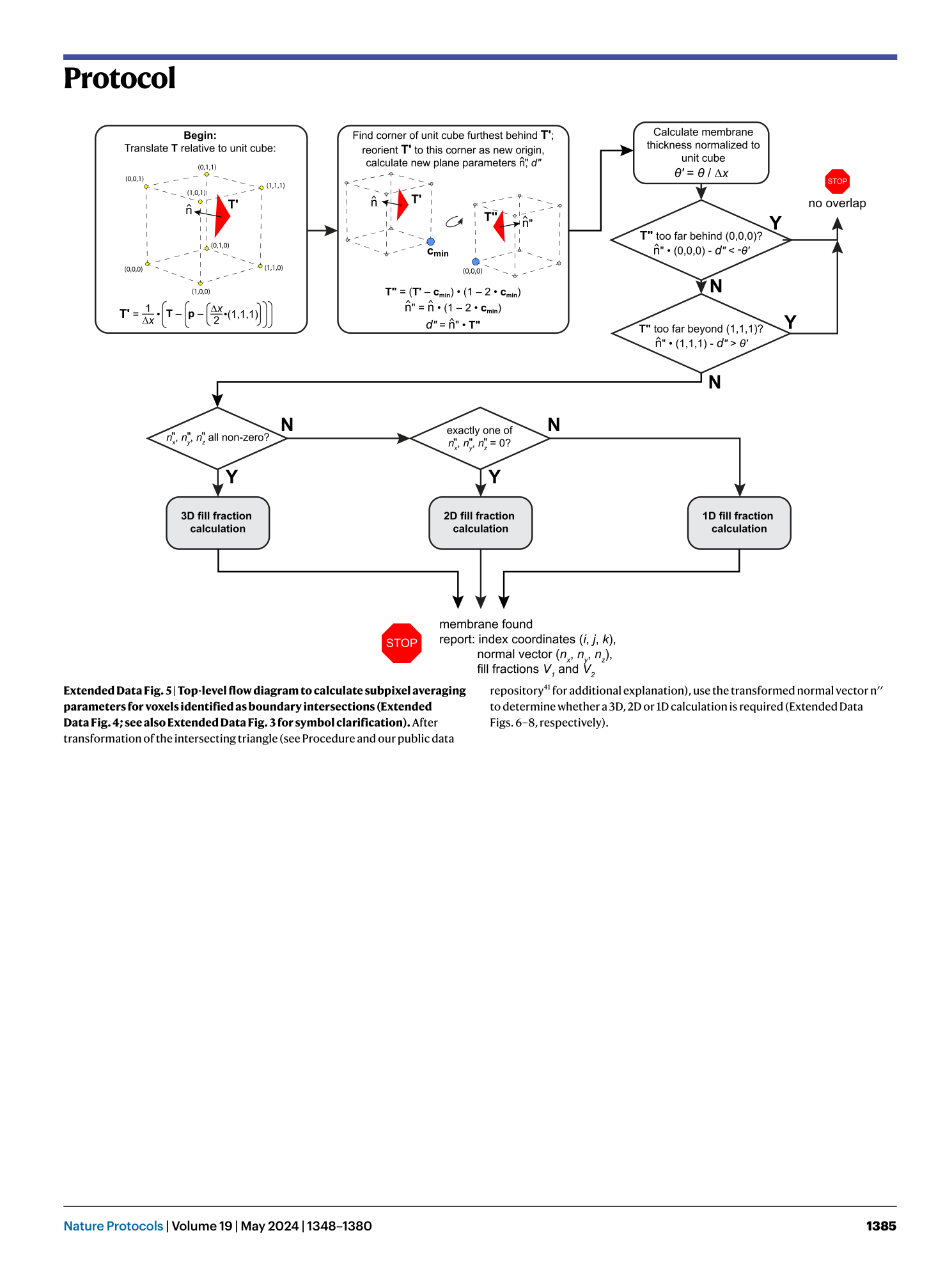
[ Extended Data Fig. 5 Top-level flow diagram to calculate subpixel averaging parameters for voxels identified as boundary intersections (Extended Data Fig. 4 ; see also Extended Data Fig. 3 for symbol clarification). ](https://www.nature.com/articles/s41596-023-00947-z/figures/14)

After transformation of the intersecting triangle (see Procedure and our public data repository 41 for additional explanation), use the transformed normal vector n′′ to determine whether a 3D, 2D or 1D calculation is required (Extended Data Figs. 6 – 8 , respectively).

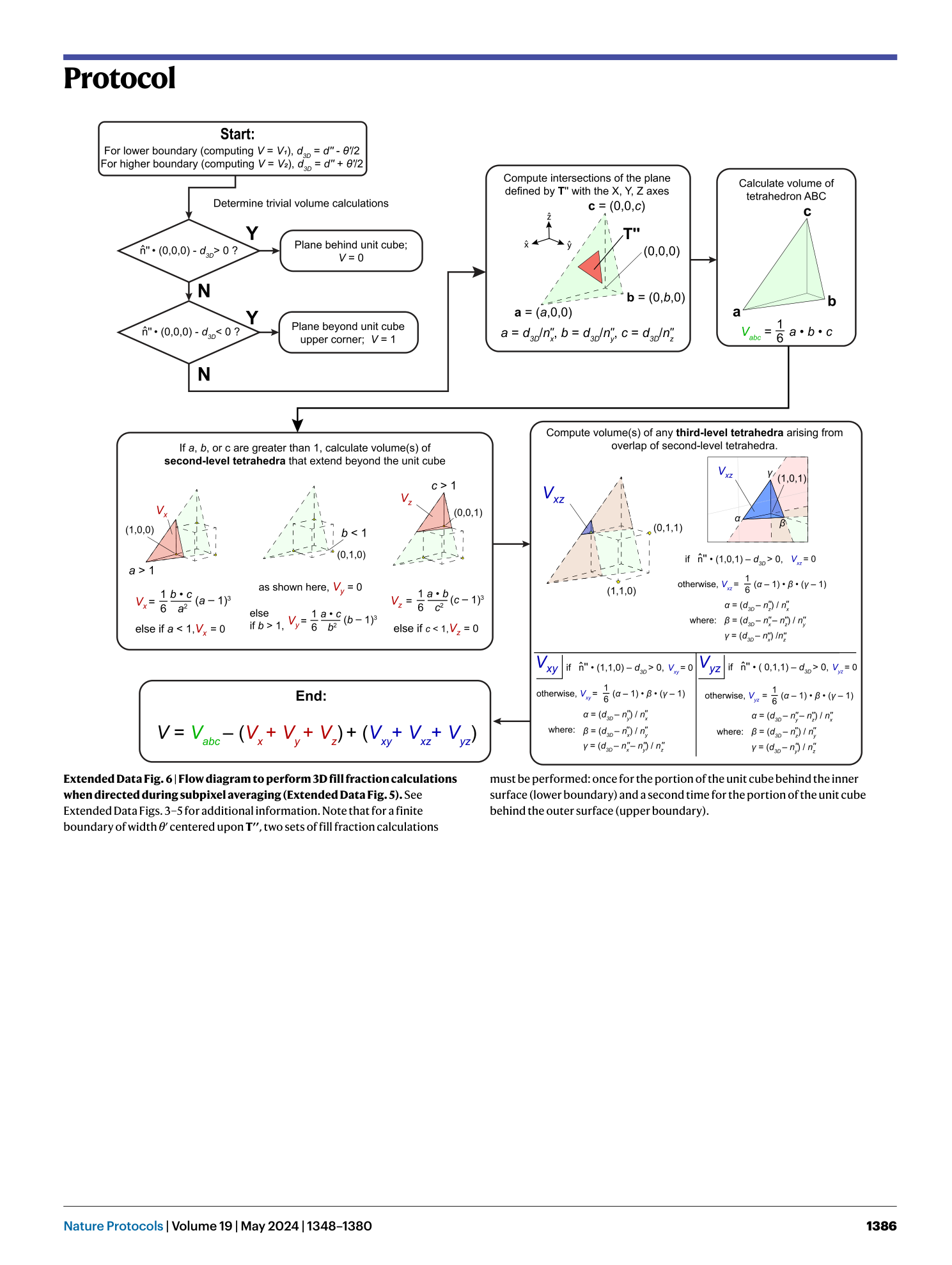
[ Extended Data Fig. 6 Flow diagram to perform 3D fill fraction calculations when directed during subpixel averaging (Extended Data Fig. 5 ). ](https://www.nature.com/articles/s41596-023-00947-z/figures/15)

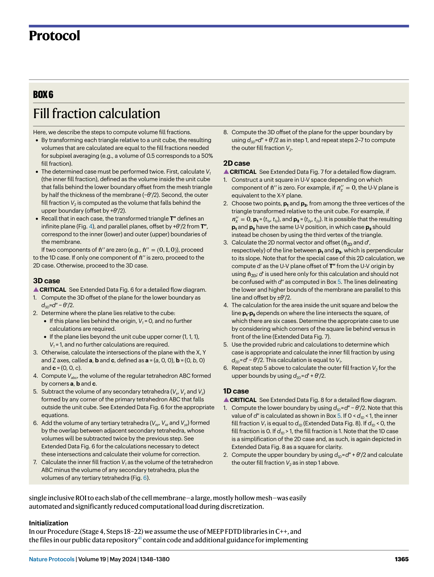
See Extended Data Figs. 3 – 5 for additional information. Note that for a finite boundary of width θ ′ centered upon T′′ , two sets of fill fraction calculations must be performed: once for the portion of the unit cube behind the inner surface (lower boundary) and a second time for the portion of the unit cube behind the outer surface (upper boundary).

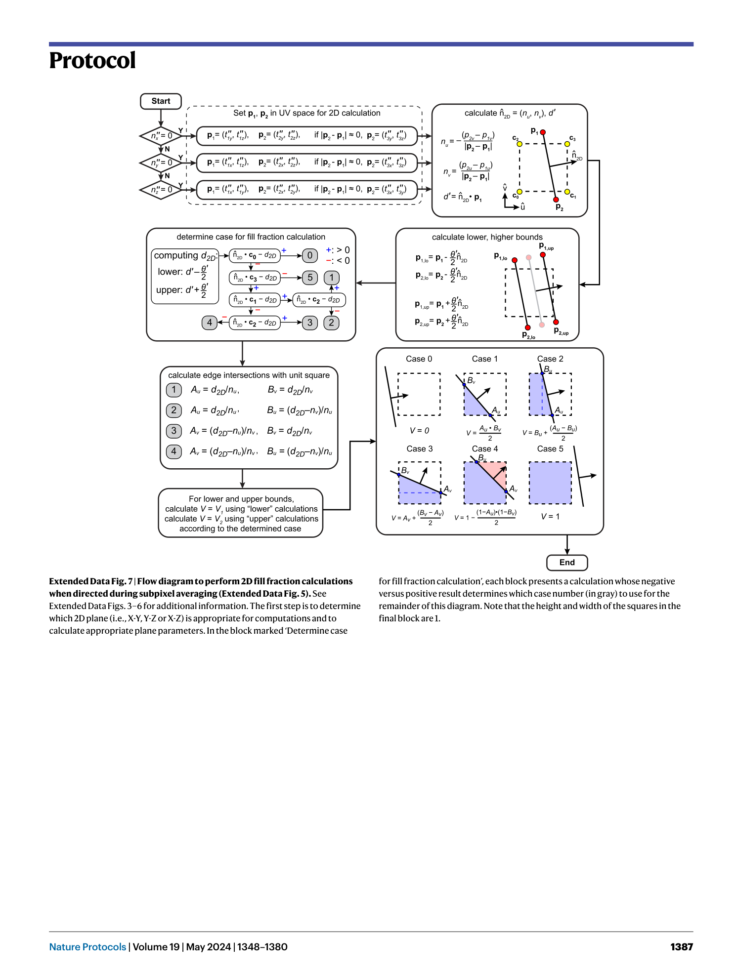
[ Extended Data Fig. 7 Flow diagram to perform 2D fill fraction calculations when directed during subpixel averaging (Extended Data Fig. 5 ). ](https://www.nature.com/articles/s41596-023-00947-z/figures/16)

See Extended Data Figs. 3 – 6 for additional information. The first step is to determine which 2D plane (i.e., X-Y, Y-Z or X-Z) is appropriate for computations and to calculate appropriate plane parameters. In the block marked ‘Determine case for fill fraction calculation’, each block presents a calculation whose negative versus positive result determines which case number (in gray) to use for the remainder of this diagram. Note that the height and width of the squares in the final block are 1.

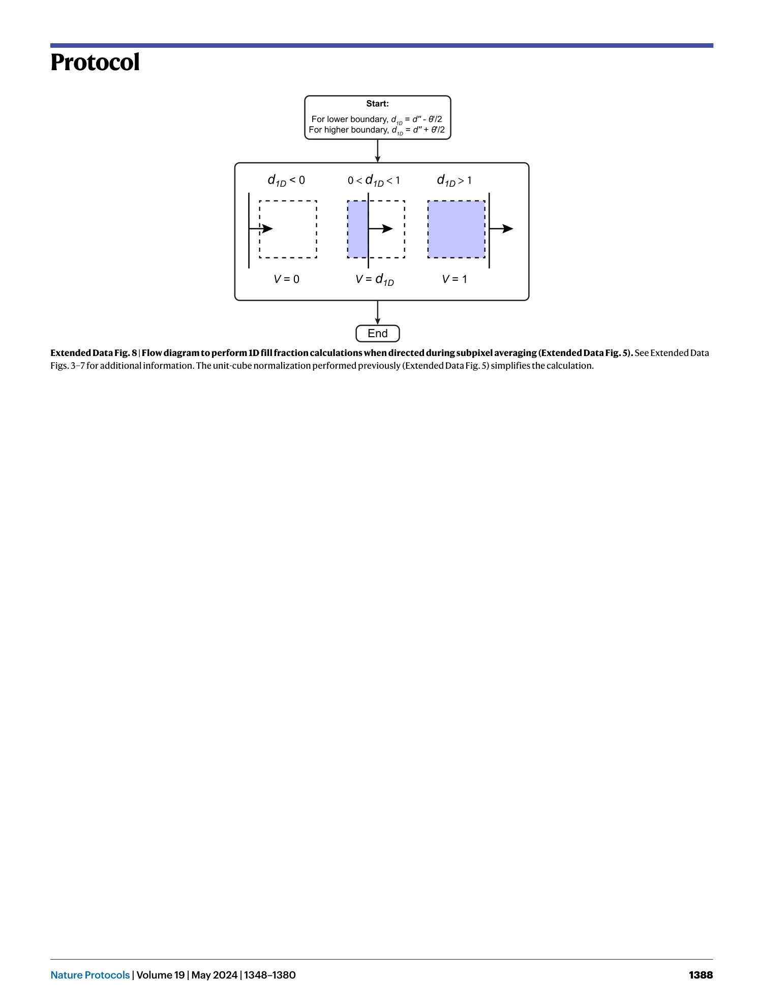
[ Extended Data Fig. 8 Flow diagram to perform 1D fill fraction calculations when directed during subpixel averaging (Extended Data Fig. 5 ). ](https://www.nature.com/articles/s41596-023-00947-z/figures/17)

See Extended Data Figs. 3 – 7 for additional information. The unit-cube normalization performed previously (Extended Data Fig. 5 ) simplifies the calculation.

Supplementary Information

Supplementary Tutorial

Supplementary Video 1

Animation depicting the use of the rigid body physics engine in Blender to fill the cone photoreceptor inner segment membrane ‘container’ with arbitrary shapes representing alternative mitochondria morphologies. The development of this model is detailed in the tutorial found in Supplementary Information.