Quantification of GTPase Cycling Rates of GTPases and GTPase:Effector Mixtures Using GTPase Glo Assays
Sophie Tschirpke, Sophie Tschirpke, Werner K.-G. Daalman, Werner K.-G. Daalman, Liedewij Laan, Liedewij Laan
Abstract
In different cellular activities such as signal transduction, cell division, and intracellular transportation, small guanosine triphosphatases (GTPases) take on a vital role. Their function involves hydrolysis of guanosine triphosphate (GTP) to guanosine diphosphate (GDP). In this article, we explain the application of a commercially available GTPase assay—the GTPase Glo assay by Promega—for investigation of GTPase-effector interactions. We provide experimental protocols together with an analysis model and software to obtain GTPase cycling rates of GTPases and GTPase:effector mixtures. GTPase cycling rates refer to the rates by which a GTPase completes an entire GTPase cycle. These rates enable quantification of the strength of GTPase effectors in a concentration-dependent fashion, as well as quantification of the combined effect of two effectors, independent of which GTPase cycle step they are affecting. © 2024 The Authors. Current Protocols published by Wiley Periodicals LLC.
Basic Protocol : Conducting GTPase Glo assays
Support Protocol 1 : Analyzing GTPase assays to correlate luminescence with remaining GTP
Support Protocol 2 : Fitting GTPase assay data to obtain GTPase cycling rates
INTRODUCTION
Small guanosine triphosphatases (GTPases) are a class of enzymes that play a fundamental role in various cellular processes, including signal transduction, cell division, and intracellular transport. GTPases regulate the hydrolysis of guanosine triphosphate (GTP) to guanosine diphosphate (GDP). Mechanistically, this activity involves three steps (Fig. 1): (1) binding of GTP to the GTPase, (2) hydrolysis of GTP to GDP and free phosphate, and (3) release of GDP from the GTPase. GTPase activity is often regulated by effector proteins: GTPase activating proteins (GAPs) that boost step 2 and GDP/GTP exchange factors (GEFs) that enhance step 3 (Bos et al., 2009; Cherfils & Zeghouf, 2013; Vetter & Wittinghofer, 2001). Several assays exist that examine single GTPase cycle steps, which helps us understand the mechanistic details of these cycle steps and their regulation. On the other hand, they do not allow study of the interplay of effectors acting on different GTPase cycle steps. Furthermore, approaches that reconstitute the complex cellular functions of GTPases in vitro (Bezeljak et al., 2020; Kohyama et al., 2022; Loose et al., 2008; Vendel et al., 2019) are sensitive to variations in protein batch activities and benefit from easy and accessible assays assessing protein purification batches activities.
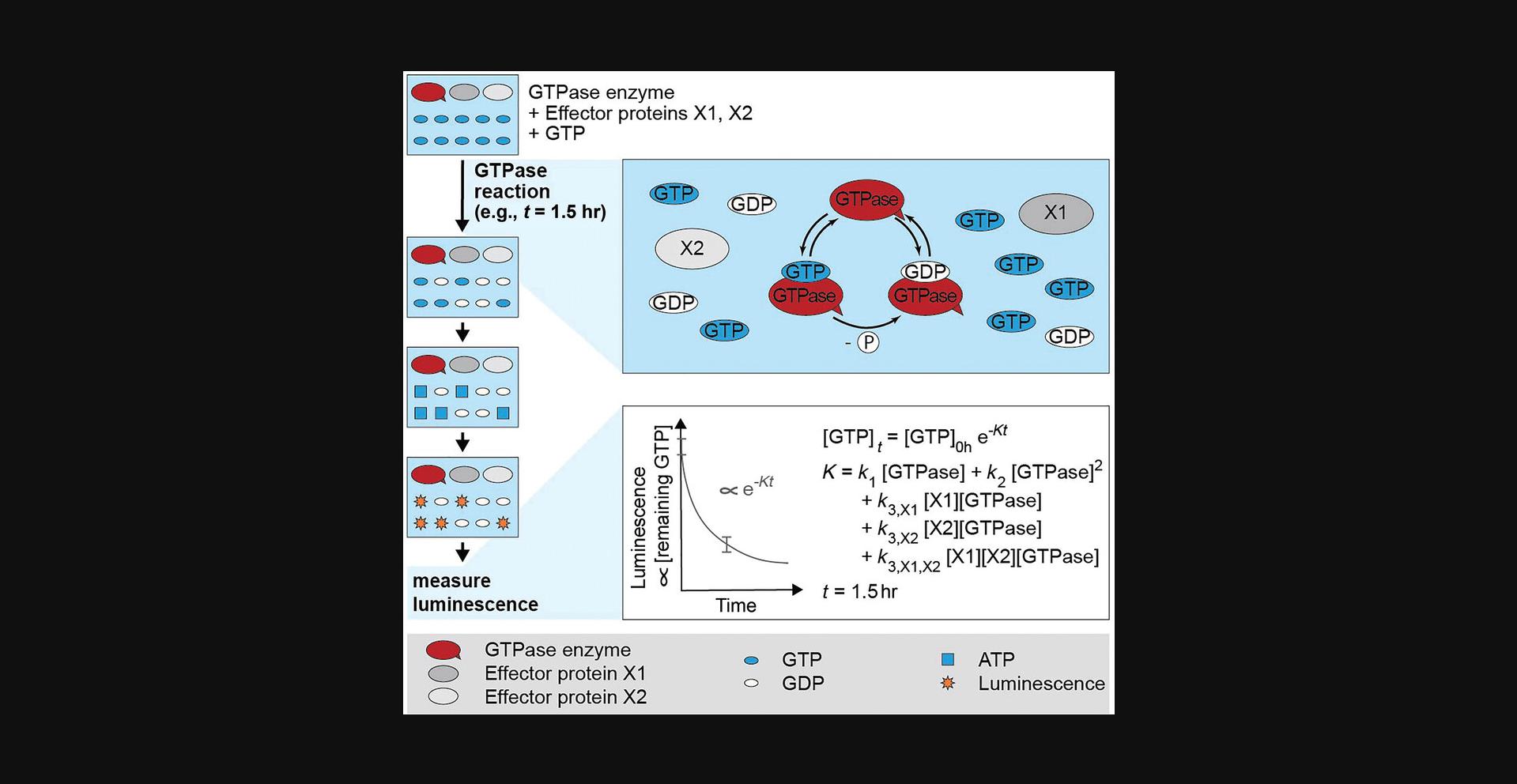
We here describe how a commercially available GTPase assay (the Promega GTPase Glo assay, henceforth referred to as the GTPase assay) can be used to quantitatively study GTPase-effector interactions and effector interplay and to easily test activity of GTPase and effector purification batches. In the GTPase assay, proteins of interest are incubated with GTP for a specified amount of time for GTPase cycling to occur. The reaction is then stopped and the amount of remaining GTP is determined as luminescence signal. GTPase cycling rates can be obtained from the resulting data using a coarse-grained exponential fitting model (Fig. 1). This article describes the workflow for conducting GTPase assays using GTPase:effector protein mixtures, and provides analysis software to obtain GTPase cycling rates. GTPase cycling rates describe the rate by which the GTPase completes entire GTPase cycles. Our protocols enable a quantitative analysis of the single and combined effect of one or two effectors on the entire GTPase cycle in a concentration-depended fashion, thus allowing the study of effectors (e.g., GEFs and GAPs) acting together on different steps of the GTPase cycle. We do not advise using this protocol if single GTPase steps are to be examined in-depth, but rather when the effects of a protein on the entire GTPase cycle are of interest. This method is illustrated using a basic GTPase assay with human Ras (GTPase) (example 1) and an elaborate GTPase assay using Saccharomyces cerevisae Cdc42 (GTPase), Cdc24 (GEF), and Rga2 (GAP) (example 2) (Tschirpke, Daalman et al., 2023). Table 1 summarizes how these examples are used to illustrate the protocols described. The protocols can be applied to other GTPases and effectors. In the Basic Protocol, we outline the workflow for conducting GTPase Glo assays. In Support Protocol 1, we describe how the GTPase assay data (luminescence) are converted to amounts of remaining GTP. In Support Protocol 2, we describe how data obtained by Support Protocol 1 can be fitted with a GTPase cycling model (and the openly available Matlab code developed by us) to obtain GTPase cycling rates.
| Example 1: Basic GTPase assay | Example 2: Elaborate GTPase assay set | |
|---|---|---|
| Experimental procedure | ||
| Basic Protocol | Based on this example | — |
| Strategic Planning | — | Features considerations absolutely necessary for this assays set (especially Fig. 2) |
| Proteins | Ras (GTPase) | Cdc42 (GTPase), Cdc24 (GEF), Rga2 (GAP) |
| Number of assays | 2 | 23 |
| Raw data | example1.xlsx (tab: ’E1’, ’E2’) | — |
| Data processing | ||
| Support Protocol 1: Calculating remaining GTP from luminescence values | Based on this example | — |
|
Input: example1.xlsx (tab: ’E1’, ’E2’) Output: same file as input |
— | |
| Reformatting of Support Protocol 1 output data to generate Support Protocol 2 input data (see Supporting Information S9) | — | |
| Support Protocol 2: Fitting GTPase cycling rates using an exponential model (see Supporting Information S8) | Based on this example | Based on this example |
|
Input: example1.xlsx (tab: ’matlab’) Assaylist-example1.xlsx |
Input: example2-matlab.xlxs Assaylist-example2.xlsx |
|
|
Output in example1 matlab output folder: Data_summary.xlsx Data_assays.mat Figure folder |
Output in example2 matlab output folder: Data_summary.xlsx Data_assays.mat Figure folder |
|
| Fitting parameters: k1, k2 | Fitting parameters: k1, k2, k3,Cdc24, k3,Rga2, k3,Cdc24,Rga2, ccorr | |
| Understanding Results | ||
| Explanation of: |
Luminescence k1, k2 Output file structure pooling of rates k |
ccorr k3,Cdc24, k3,Rga2, k3,Cdc24,Rga2 Comparison of rates |
- a Data files available at data.4tu.nl (see Data Availability).
STRATEGIC PLANNING
If the GTPase assay is being performed for the first time, we advise first practicing the pipetting of the small volumes required into the wells using colored water. It is best to conduct smaller assays using a larger number of replicates per sample (e.g., eight sample rows per assay with five replicates each, as described in the Basic Protocol) before moving on to larger assay sets with more proteins.
Once you feel more comfortable with the assay, larger assay sets can be conducted, for example, to look at the interaction between a GTPase and one or several effectors (e.g., GTPase-GEF, GTPase-GEF-GAP). The following section applies predominantly (but not solely) to such larger assays sets involving multiple GTPases and/or effector proteins (example 2). We advise users to determine how many proteins will be assayed well before starting the assays. Specifically, we recommend the following steps.
1.Verify that the proteins and protein buffers do not interfere with the assay signal. The GTPase assay measures luminescence, which correlates with the amount of remaining GTP. Proteins that interact with and can alter luminescence (e.g., fluorescent tags, see Supporting Information S3) are therefore not suitable for this assay. Buffers containing ADP, ATP, GDP, GTP, and guanosine phosphate analogs are also not suitable, as they interfere with GTPase assay step reactions. Consider the buffer components carefully and verify that the effector proteins used do not exhibit GTPase activity.
2.Verify that incubation times lie in the exponential decline region of the remaining GTP. In the GTPase assay, the proteins of interest are incubated with GTP for a specified amount of time during which GTPase cycling can occur. The reaction is then stopped and the amount of remaining GTP is determined as a luminescence signal. GTPase cycling rates can be obtained from these data through a coarse-grained exponential fitting model (Fig. 1 and Supporting Information S8). The model is based on our observation that the amount of remaining GTP declines exponentially with time (Supporting Information S4). It is advisable to verify that this is true for the proteins being studied (GTPase enzymes and GTPase:effector mixtures) and incubation times to be used. To obtain such data, prepare one batch of serial dilutions of the proteins you will use. Use exactly these dilutions to conduct several assays with different incubation times. Check whether the amount of remaining GTP in these assays follows an exponential decline. Further, analyze each assay individually using our GTPase cycling model. Verify that different incubation times (different assays) yield the same rates (e.g., Supporting Information S4).
3.Dialyze all proteins in same buffer. In the assay, protein activity is determined by normalizing the assay readout (luminescence) to a well containing buffer only. Thus, differences in ion concentrations, detergents, or other additives (such as glycerol) can lead to differences in luminescence. This is easily avoided if all proteins used in an assay set are prepared in the same buffer. We advise against using a buffer containing glycerol, as the increased viscosity may affect protein activities (unless protein activities in a denser environment are of interest). Further, buffers should not contain DTT; GDP, GTP, or other guanosine analogs; ADP, ATP, and other nucleotide triphosphates; or EDTA or other chelating agents that can complex magnesium. If a GTPase-GEF interaction is to be investigated, the buffer usually requires magnesium salts (e.g., 10 mM MgCl2).
Many proteins require glycerol for storage. In this case, keep the protein at a high concentration (at least six times of the concentration that ought to be used in the assay) in a buffer containing glycerol (e.g., 50 mM Tris-HCl, pH 7.5, 100 mM NaCl, 10 mM MgCl2, 1 mM 2-mercaptoethanol, 10% glycerol) and then dilute it into the same buffer without glycerol. GTPase assays usually require small concentrations of proteins (in our experience, 0.5-5 µM). If the protein is stored at a high concentration, the amount of glycerol in the final reaction will be negligible.
If it is not possible to prepare all proteins in the same buffer, one must verify that the differences in buffer composition do not affect luminescence intensities. A GTPase assay containing only the different buffers can elucidate this. If all buffer mixtures exhibit the same luminescence values, then the differences in buffer composition do not affect luminescence. It should be noted that it is still possible that the buffer components affect protein behavior.
4.Use the same serial dilution for all assays. The assay is sensitive to concentration changes, especially for highly active GTPases and effectors that strongly boost GTPase activity, and thus is also sensitive to pipetting errors when preparing protein dilutions. Prepare serial dilutions of every protein and use exactly the same serial dilution for the entire assay series (Fig. 2). Different serial dilutions of the same protein can exhibit slightly different rates. For example, when comparing the effect of effector protein X on GTPase A and GTPase B, the same serial dilution of effector X must be used for both GTPases.
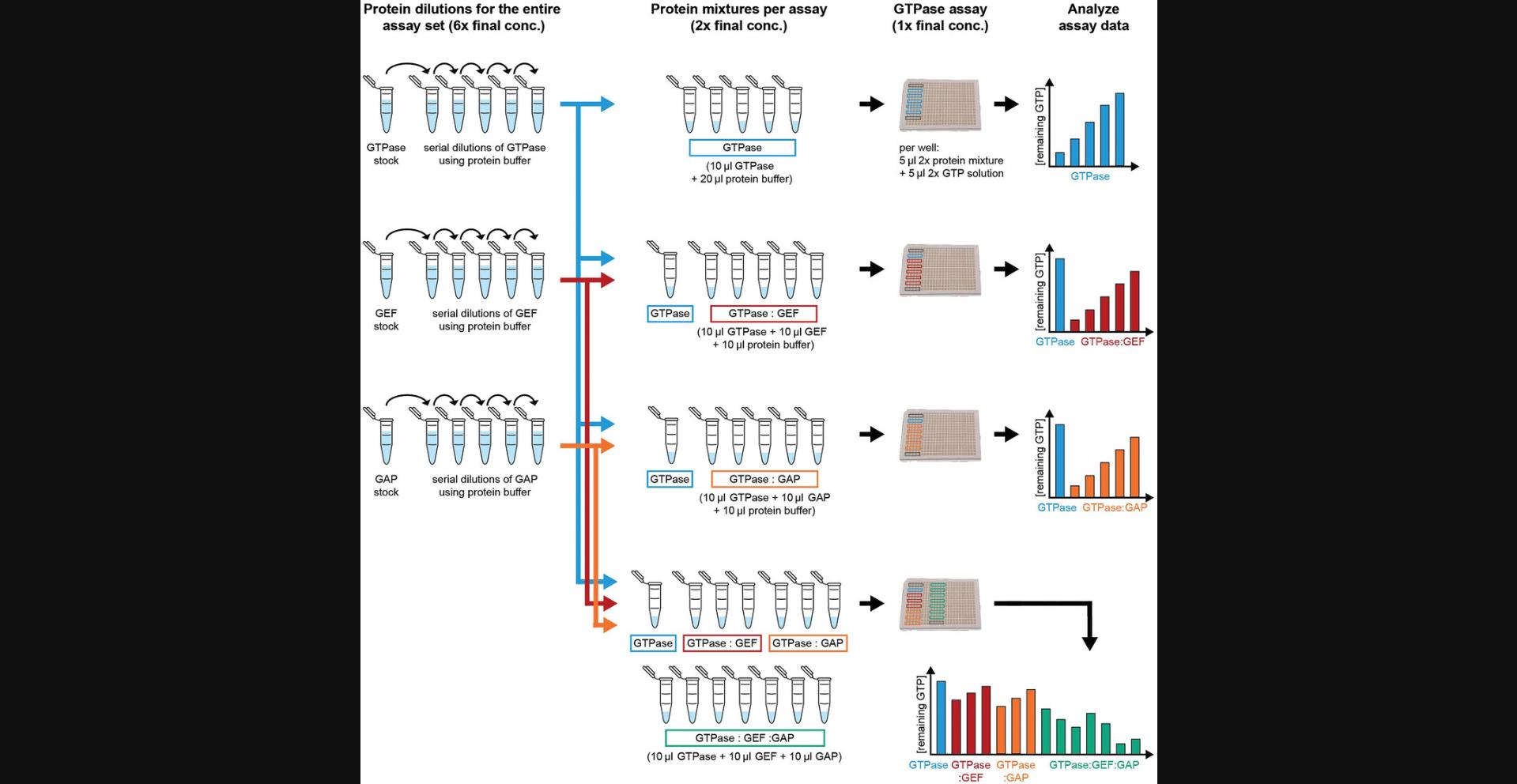
5.Include a reference sample if data from different assays will be compared. GTPase assays can be sensitive to GTPase activity changes resulting, for example, from small pipetting errors or changes in conditions (e.g., temperature, shaker speed). As this can lead to slight changes in protein activity between assays, it is best to include all samples to be compared in the same assay. This is not always possible. If the strength of several effectors on one GTPase will be compared, we recommend always including one sample containing only the GTPase in each assay (Fig. 2). The assay-specific activity of the GTPase sample can then be used to account for any assay-specific variability (through fitting the correction factor c corr, as will be explained in Support Protocol 2 and in Eqn. 9 of Supporting Information S8). Assay variations are typically very small (reflected as c corr ≈ 1.0) (Tschirpke, Daalman et al., 2023; Tschirpke, van Opstal et al., 2023). We recommend excluding assays that show vastly different protein activities (reflected in a c corr much larger or much smaller than 1), as these indicate that the GTPase behavior/assay conditions are unusual.
6.Determine useful concentration ranges before conducting an assay series. In our experience, a good readout regime is 5%-90% remaining GTP. Higher values (>90% remaining GTP) have a larger error (due to normalization) and lower values (<5% remaining GTP) may show a saturation effect due to the small amount of remaining GTP. In the recommended regime, a saturation of the fitted cycling rates may occur. If an assay with multiple proteins (e.g., a GTPase and two effector proteins) is conducted, it is useful to determine beforehand which concentration ranges of each protein lead to optimal readouts to reduce the time it takes to conduct the entire assay series. It is also advisable to stick to similar incubation times for all assays, as this streamlines the selection of protein concentrations (for assays containing protein mixtures) that yield suitable readout regimes.
7.Make an assay plan. Use the same serial dilutions when quantifying and comparing multiple protein interactions. Since many proteins are not stable for weeks at room temperature or 4°C and require glycerol for cryopreservation (which is not recommended), all required assays must be conducted within a rather short time period to obtain reliable and comparable results. We strongly recommend careful planning of which assays will be conducted using which proteins, and calculating the required volumes of protein needed. Our recommended procedure is explained below using as an example a GTPase assay series investigating the cycling of a GTPase and the effects of both a GEF and a GAP, alone and in combination (example 2; Fig. 2; Tschirpke, Daalman et al., 2023).
Considerations (as described earlier) : (1) Different serial dilutions of the same protein may exhibit slightly different rates due to small pipetting errors. Hence, the same dilution should be used for the entire assay set. (2) For larger assays, it is advisable to know in advance which concentration ranges give good signal to reduce the time the proteins need to be stored. (3) A reference sample should be included (a sample of the GTPase alone, at the concentration used in the particular assay). (4) The incubation times used should be in the exponential region. (5) It is advisable to use similar incubation times for all assays, as this will make it easier to choose protein concentrations for assays containing protein mixtures that will result in suitable readouts.
Protein dilutions : To conduct the assay, protein dilutions are needed for the three proteins used in the entire assay set (GTPase, GEF, and GAP; Fig. 2, left column). These dilutions will be used to create the protein mixtures for one GTPase assay (Fig. 2, middle column). The concentration of the dilutions depends on two factors: (1) The number of protein species in the assay (N). For a mixture containing a GTPase, GEF, and GAP, N is 3.As it is easiest to prepare the various mixtures by combining proteins in 1:1:1 volume ratios, each protein will be diluted by a factor of three in setting up the assay. (2) To initiate the GTPase reaction, a 2× GTP solution is mixed in a 1:1 volume ratio with each protein mixture. Together, the protein dilutions (left column) should be prepared at a 2× N -fold higher concentration than the final concentration in the assay (right column). Thus, for an assay set with a GTPase, GEF, and GAP, all protein dilutions should be prepared at 6× concentration. For assay sets investigating mixtures of four or five proteins, N will be 4 or 5 and the dilutions must be 8× or 10×, respectively.
Procedure : First, an assay is conducted with a serial dilution of only the GTPase (Fig. 2, top row). From this assay, pick one or two GTPase concentrations to conduct all subsequent assays. Because the subsequent assays involve a GEF and a GAP, both of which boost GTPase activity, it is wise to choose a GTPase concentration that leads to a high amount of remaining GTP (e.g., 80%-90%). Next, an assay is conducted with the chosen concentration of GTPase and a serial dilution of the GEF (Fig. 2, second row). A similar assay is conducted with GTPase and the GAP (Fig. 2, third row). Finally, an assay is conducted with all three proteins in multiple combinations (GTPase alone, GTPase:GEF, GTPase:GAP, and GTPase:GEF:GAP) all using the same GTPase concentration. For this final assay, choose GEF and GAP concentrations that resulted in a medium amount of remaining GTP (e.g., 60%-70%) to leave room for even lower values when both proteins are combined (Fig. 2, bottom row). Ideally, additional assays will be added to control for potential non-canonical effects (see below).
8.Control for non-canonical effects by adding an inert protein. We have observed several potential artefacts during GTPase cycling in this assay. These effects are generally small and can be accounted for. For example, we observed that both bovine serum albumin (BSA) and casein cause a slight boost in GTPase activity of both Ras and Cdc42.BSA and casein are considered inert and have no known interaction with either Ras or Cdc42. We suspect that they seemingly boost GTPase activity by increasing the effective GTPase concentration. A few GTPase molecules might stick to the well in each reaction chamber, being rendered inactive. When another protein is added, the chamber wall will be covered with some molecules of both GTPase and the other protein, thereby increasing the effective GTPase concentration. To ensure that the effect of a protein on GTPase cycling is not only due to these non-canonical effects, we advise conducting additional assays with the GTPase and an inert protein (e.g., BSA or casein). The effect of the protein of interest will need to exceed that of an equimolar concentration of the inert protein to be of non-canonical origin. It should be noted that BSA is strongly negatively charged, which could lead to non-specific protein interactions. Therefore, casein might be more suitable as a control. For example 2 with a GTPase, GEF, and GAP (Fig. 2), control assays for non-canonical effects include: (1) GTPase:casein serial dilution, (2) GTPase:GEF:casein, and (3) GTPase:GAP:casein.
Basic Protocol: CONDUCTING GTPase Glo ASSAYS
In the GTPase Glo assay, proteins of interest (GTPase enzymes with or without effectors) are incubated with GTP for a specified amount of time for GTPase cycling to occur (Fig. 1). Once the reaction is stopped, the remaining GTP is translated into a luminescence signal and measured. The following steps are from the assay manual with only minor modifications. The volumes provided are for assays in 384-well microplates. Assays using larger volumes can be conducted using different plates (see the assay manual). In addition to following the steps here, we recommend carefully reading the assay manual.
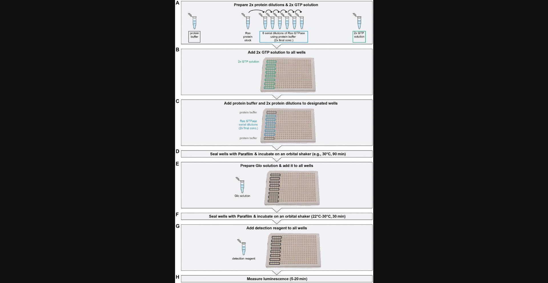
The following steps are for a GTPase assay with a serial dilution for six concentrations of Ras GTPase (example 1; Fig. 3). An illustration of the required assay planning steps is shown in Supporting Information S2.The assay results in data that are found in example1.xlsx, tab: ’E1’, ’E2’.
Materials
-
Proteins of interest:
- GTPase (e.g., human Ras, EMD Millipore, cat. no. 553325)
- Optional effector proteins (GEP, GAP)
-
Protein buffer: 50 mM Tris-HCl, pH 7.5, 100 mM NaCl, 10 mM MgCl2, 1 mM 2-mercaptoethanol
-
Inert protein (optional): casein (Sigma-Aldrich, cat. no. C7078) or bovine serum albumin (BSA; Thermo Scientific, cat. no. 23209)
-
GTPase Glo assay (Promega, cat. no. V7681 or V7682 for 1,000 or 10,000 reactions)
-
384-well white, flat-bottom microplates (Corning, cat. no. 3572)
-
Parafilm
-
1.5- and 15-ml reaction tubes
-
Orbital shaker (e.g., Innova 2300 platform shaker, New Brunswick Scientific)
-
Temperature-controlled incubator (optional)
-
Plate reader to measure luminescence (e.g., Synergy HTX, BioTek)
Prepare protein
1.Dialyze GTPase in protein buffer following the instructions accompanying the chosen dialysis device.
Prepare for assay (mise-en-place)
Before beginning, decide on the assay scope and prepare all materials needed. For templates, see Supporting Information S1; for an example assay using Ras GTPase, see Supporting Information S2 and Figure 3.
2.Decide which samples and how many replicates are needed.
3.Calculate the volumes (V) of protein dilutions, 2× GTP solution, Glo solution, and detection reagent needed to conduct the assay (for example calculations, see Supporting Information S2).
- V prot = 5 µl × number of replicates
- V GTP = 5 µl × number of replicates per sample × number of samples
- V Glo = 2 × V GTP
- V det = 4 × V GTP
4.Calculate the dilution series steps for the GTPase, keeping in mind that the solutions must be 2× the final concentration in the assay (for example calculations, see Supporting Information S2).
5.Set up the 384-well assay plate as in Figure 3C. Label wells that will be used in the assay and seal wells that will not be used with Parafilm to prevent contamination with dirt.
-
For one assay, designate five columns of a 96-well plate to give five replicates per sample.
-
Arrange the two protein buffer samples in the top and bottom rows of the plate.
In rare cases, luminescence values drift slightly towards lower values throughout the assay. Placement of a buffer row as the first and last rows ensures that this drift can be detected and be accounted for in the analysis.
-
Arrange the six GTPase dilutions between the buffer rows.
-
Leave an empty row between all buffer/sample rows.
6.Cut four pieces of Parafilm that are big enough to cover the area used for the assay.
Conduct assay
7.Thaw protein samples and assay solutions on ice.
8.Make six 2× serial dilutions of GTPase with protein buffer according to your calculations (Fig. 3A). Vortex to mix and spin down gently to collect all volume at the bottom of the tubes.
9.Prepare the 2× GTP solution (Fig. 3A). Vortex the GTP and DTT stock solutions, then combine as then combine with protein buffer according to Table 2 and vortex again.
| Volume | ||||
|---|---|---|---|---|
| Reagent | Final concentration | For 500 μl | For 750 μl | For 1 ml |
| Protein buffer | — | 494 μl | 742 μl | 989 μl |
| 100 mM DTT | 1 mM | 5 μl | 7.5 μl | 10 μl |
| 10 mM rGTP | 10 μM | 0.5 μl | 0.75 μl | 1 μl |
10.Add 5 µl of 2× GTP solution to all wells (Fig. 3B).
11.Add 5 µl protein buffer and 2× GTPase dilutions to the designated wells (Fig. 3C).
12.Seal wells with two sheets of Parafilm and incubate for the designated time on an orbital shaker.
13.Several minutes before the incubation is finished, prepare the Glo solution (Fig. 3E).
-
Vortex Glo buffer and 10 mM ADP to mix.
-
Tap the tube of Glo reagent to mix (donotvortex).
-
Dilute 10 mM ADP to 1 mM using ultrapure water. Vortex to mix.
-
Combine reagents according to Table3and vortex to mix.
| Volume | ||||
|---|---|---|---|---|
| Reagent | Final concentration | For 500 μl | For 750 μl | For 1 ml |
| GTPase-Glo buffer | — | 496 μl | 745 μl | 993 μl |
| 1 mM ADPa | 5 μM | 2.5 μl | 3.75 μl | 5 μl |
| 500× GTPase-Glo reagent | 1× | 1 μl | 1.5 μl | 2 μl |
-
aThe ADP solution provided in the kit must first be diluted from 10 mM to 1 mM (e.g., mix 2 μl of 10 mM ADP with 18 μl ultrapure water).
14.At the designated time, add 10 µl Glo solution to all wells (Fig. 3E), seal with two sheets of Parafilm (as above), and incubate 30 min at room temperature on an orbital shaker.
15.Add 20 µl detection reagent to all wells (Fig. 3G).
16.Measure luminescence of each well using a plate reader for 20 min.
Support Protocol 1: ANALYZING GTPase ASSAYS TO CORRELATE LUMINESCENCE WITH REMAINING GTP
This protocol describes basic analysis steps to calculate the amount of remaining GTP from the GTPase assay readout (luminescence). The amount of remaining GTP is a simple measure used to compare the activity of different GTPases (of the same concentration, incubated with GTP for the same amount of time). The protocol illustrates steps for example 1: an assay including six Ras GTPase serial dilutions and two buffer reference samples (see Basic Protocol and Supporting Information S2), with three replicates each. The protocol uses and generates data in example1.xlsx, tab: ’E1’, ’E2’. A spreadsheet editor or other analysis software is needed. The provided Python script (see Supporting Information S9) is needed if cycling rates will also be determined.
Calculate remaining GTP and its error
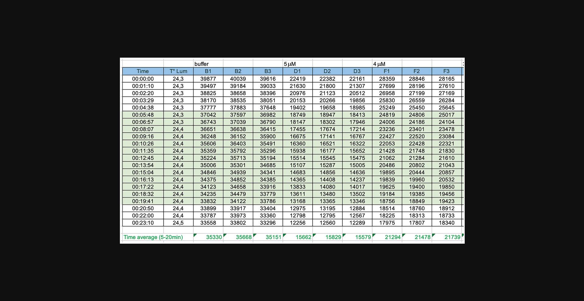
1.Calculate the average luminescence for all time points from 5 to 20 min for each well (Fig. 4).
2.Calculate the average luminescence for each sample (Lums) by averaging the wells (replicates) for that sample (Fig. 5, row a).
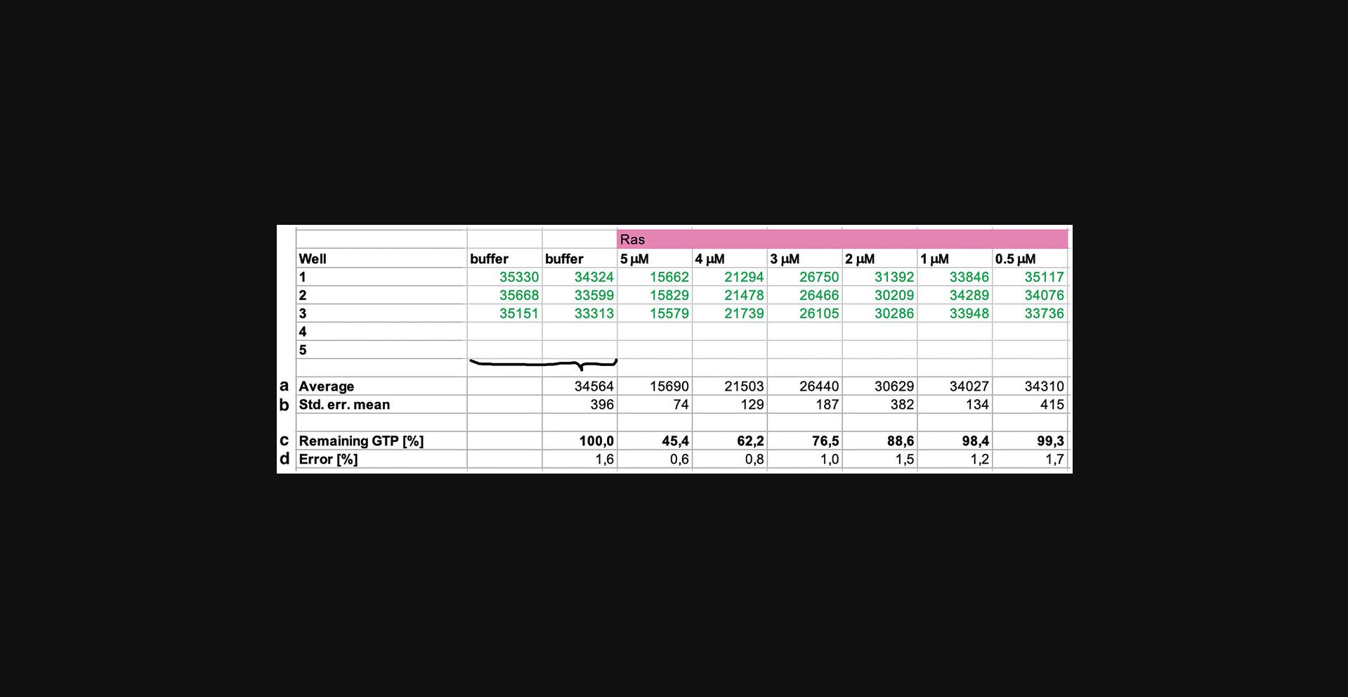
3.Calculate the average luminescence for protein buffer (Lumb) by averaging the wells/replicates from both buffer rows in a single calculation (Fig. 5, row a). Do not distinguish between the first and last buffer row.
4.Calculate the standard error of the mean for each sample and buffer (ΔLums and ΔLumb) (Fig. 5, row b).
5.Use the average luminescence values to calculate the amount of remaining GTP (Fig. 5, row c) using the equation:
6.Calculate the error (Δ remaining GTP; Fig. 5, row d) by error propagation using the equation:
Format data for subsequent analysis (optional)
This process is only required if the data analysis will be continued to determine GTPase cycling rates in Support Protocol 2.It involves organizing the data in a spreadsheet with a specific format (Fig. 6) and the following column headers:
- Run = assay number. This must consist of an E followed by a number, which can be followed by letter(s) with or without an underscore. For example: E1, E2, E100, E1a, E100abc, E1_a, E100_abc, E1a_abc, E100f_abc
- Time = incubation time. Values must be in hours.
- GTP_remaining = amount of remaining GTP normalized to 1
- Error = error values normalized to 1
- Buffer_error: error of buffer normalized to 1
- [GTPase]_conc = name of the GTPase followed by ‘_conc’ (e.g., Ras_conc in Fig. 6). Values must be in µM.
- [Effector]_conc (optional) = name of the effector followed by ‘_conc’. Values must be in µM. This column should only be present if it contains more than one unique value per assay.
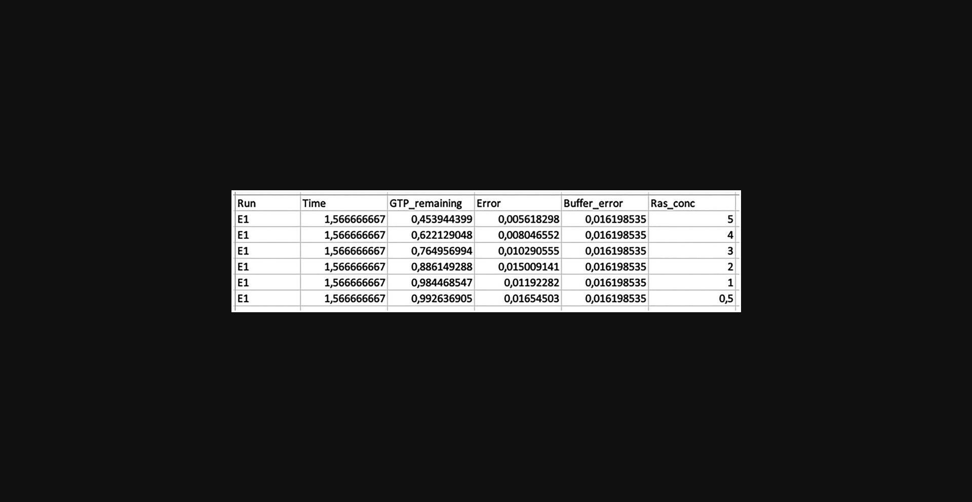
Reformatting the data can be done using the Python script Ras_example.ipynb (see Supporting Information S9). For example 1, the steps are:
7.Open Ras_example.ipynb and state the input data and relevant tab names:
- datafilename = ’example1.xlsx’
- tabnamelist = [’E1’,’E2’]
8.Run the Python script to generate two Excel sheets: ’E1.xlsx’ and ’E2.xlsx’.
9.Copy data from both outputs into a single Excel sheet, but include only one header (see first figure in Supporting Information S9). This will be the input for the Matlab script used in Support Protocol 2.
10.Use the find/replace option of the spreadsheet editor to replace all points (.) with commas (,).
Support Protocol 2: FITTING GTPase ASSAY DATA TO OBTAIN GTPase CYCLING RATES
This protocol describes how the data (preprocessed in Support Protocol 1) can be fitted using a GTPase activity model (see Supporting Information S8) to obtain GTPase cycling rates k , which describe the rate with which a GTPase completes GTPase cycles. It can be used to fit data of GTPases and GTPase:effector mixtures (with up to two effectors, X1 and X2).
In short, data from the GTPase serial dilutions are first fitted with an exponential to obtain GTPase cycling rates k 1 and k 2:
where K refers to the overall GTP hydrolysis rate and depends on the concentration of the GTPase. We call the concentration-independent rates (k) GTPase cycling rates, referring to the fact that they describe GTPase cycling and not specific GTPase cycle steps. The overall hydrolysis rate K is composed of an unaided hydrolysis contribution by an individual GTPase (K* 1) and a cooperative contribution by two GTPase molecules (K* 2).
Next, mixtures of one GTPase and one effector (X1) are fitted with:
Note that, in order to analyze GTPase:effector mixtures, k 1 and k 2 must be known. It is thus required to fit the data of GTPase (serial) dilutions first. The model allows one to fit GTPase:effector mixtures with up to two effectors, with each effector showing either a linear or quadratic concentration dependence. If the effectors show neither of these concentration dependencies (e.g., due to saturation), we advise either including only the linear/quadratic regimes into the analysis or extending the fitting model to match the specific case. With the provided software, it thus is possible to fit the following protein (mixtures):
- GTPase serial dilution (example 1)
- GTPase + effector serial dilution (linear or quadratic conc. dependence, Eqn. 2) (example 2)
- GTPase + effector X1 serial dilutions + effector X2 serial dilutions (Eqn. 3) (example 2, Fig. 2)
The model is based on our observation that the amount of remaining GTP declines exponentially with time (see Supporting Information S4). It is advisable to verify that this is true for the proteins (GTPase and effectors) and incubation times to be used.
The model code analyzes data of each GTPase assay individually and then generates pooled rate values (for details on weighting of k for pooling and error propagation, see Supporting Information S11). The analysis code allows one to exclude GTPase assays from pooling if c corr values or standard errors of are out of range. Decision criteria are set in the code using two parameters:
conc_corr_bounds states which range of c_corr allows assays to be included in the pooling.
k_low_err_filt.’GTPase-name’ states whether assays containing the particular GTPase that have low standard errors (1–10 or lower) for k values are excluded from pooling. This parameter must be declared individually for each GTPase.
Below, we first describe the general protocol steps (case 1), which we then apply to example 1 (a simple assay containing one GTPase) (case 2) and example 2 (an elaborate assay set containing assay data for the GTPase alone and GTPase:GEF, GTPase:GAP, and GTPase:GEF:GAP mixtures) (case 3). Finally, we provide analysis steps for the combined analysis of example 1 and example 2 data (case 4).
Necessary resources
- Spreadsheet editor
- Matlab software license, analysis scripts, and example data files encompassing this protocol
Case 1: General procedure
1a. Set up the Matlab environment. To run the code, ensure that all required files are present:

2a. Define the processing of the data in the assaylist.xlsx spreadsheet. Follow the formatting provided in the example files (discussed below in the steps of cases 2-4). The following sections are required:
- Assay name: State an internal assay name that will be used in the output to refer to these data.
- Proteins: State the names of proteins whose concentration varies within the assay (maximum of two proteins per assay). State each protein in a separate column.
- GTPase ref.: State the assay name where the GTPase was varied. Ensure that this assay has already been processed (i.e., is earlier in the list).
- Data file location: State the relevant file location.
- Relevant tab names: State which tab of the data file should be used.
3a. Open Process_assays.m. Define the input parameters and processing options:
- %% Input parameters
-
- AssayListName = ’ .xlsx’;
- % State the assaylist file name
-
- GTPases = {’ ’};
- % state proteins (that are stated in the assaylist file) that are GTPases
-
- LinFitEffector = {’ ’};
- % state proteins X (that are stated in the assaylist file) that should be
- % fitted with a linear fit: k_3,X [GTPase] [X]
-
- QuadFitEffector = {’ ’};
- % state proteins X (that are stated in the assaylist file) that should be
- % fitted with a quadratic fit : k_3,X [GTPase] [X]^2
- act_corr = true(1);
- % Logical to determine whether terms in the rate equation that depend on
- % GTPase] are corrected for run-specific GTPase activity/concentration
- % differences
-
- num_draws = 1e5;
- % Number of random draws from distribution of rate parameters k
-
- plot_fits = true(1);
- % Logical indicating whether fits should be outputted in .pdf and .tiff
- % (false is faster)
-
- print_fits = true(1);
- % Logical indicating whether fit results should be printed in the command window
-
- GTP_filt = true(1);
- % Logical indicating whether data points 0.00 − 0.05 % GTP remaining
- % should be disregarded for the fits
-
- conc_corr_bounds = [0.5 1.5];
- % Two−element vector that states a c_corr lower and upper bound. Assays that
- % have c_corr values within this range will be included in pooling of
- % estimates. [0 Inf] means assays with any c_corr value will be included.
- % We recommend [0.5 1.5]: assays with c_corr values from 0.5 to 1.5 will be
- % included.
-
- k_low_err_filt.’GTPase−name’ = false;
- % Logical that states per GTPase whether to discard runs from pooling that
- % have very low standard errors (1 e−10 or lower) on the k values.
- % I f nothing i s provided for a GTPase, default is true (i.e. runs with low
- % standard errors will be excluded).
4a. Run Process_assays.m.
Case 2: Simple assay with Ras GTPase (example 1)
We here show the specific protocol steps to run data for example 1, a GTPase assay containing only serial dilutions of Ras GTPase that was conducted twice. For assay steps, see Basic Protocol and Supporting Information S2. For basic analysis of the assay data, see Support Protocol 1, Supporting Information S9, and the resulting data in example1.xlsx, tab: ’matlab’.
The data for each individual assay will be fitted with the model:
- [GTP]t = [GTP]0h exp(– Kt)
- using [GTP]0h = 1 and
- K = K 1 + K 2 = k 1c corr[Ras] + k 2(c corr[Ras])2
resulting in k 1 and k 2 for each assay. A pooled estimate of k 1 and k 2 will be generated.
1b. Set up the Matlab environment. To run the code, ensure that all required files are present:

2b. Define the processing of the data in the assaylist-example1.xlsx spreadsheet:

3b. Open Process_assays.m. Define the input parameters:
- AssayListName = ’Assaylist-example1.xlsx’;
- GTPases = {’Ras’};
- LinFitEffector = {’ ’};
- QuadFitEffector = {’ ’};
- act_corr = true(1);
- num_draws = 1e5;
- plot_fits = true(1);
- print_fits = true(1);
- GTP_filt = true(1);
- conc_corr_bounds = [0.5 1.5];
- k_low_err_filt.Ras = false;
4b. Run Process_assays.m.
Case 3: Elaborate assay set with GTPase:effector mixtures (example 2)
Here we show the specific protocol steps to run data for example 2, which entails data (example2.xlsx) using the following conditions (Fig. 2):
- (A) Serial dilutions of the GTPase Cdc42 (in tab ’dCdc42’).
- (B) Constant Cdc42 concentration and serial dilutions of the GEF Cdc24 (in tab ’Cdc42-dCdc24’).
- (C) Constant Cdc42 concentration and serial dilutions of the GAP Rga2 (in tab ’Cdc42-dRga2’).
- (D) Constant Cdc42 concentration and serial dilutions of both Cdc24 and Rga2 (in tab ’Cdc42-dCdc24-dRga2’).
The data from each individual assay will be fitted with the following model based on Eqn. 3:
1c. Set up the Matlab environment. To run the code, ensure that all required files are present:

2c. Define the processing of the data in the assaylist-example2.xlsx spreadsheet:

3c. Open Process_assays.m. Define the input parameters:
- AssayListName = ’Assaylist-example2.xlsx’;
- GTPases = {’Cdc42’};
- LinFitEffector = {’Rga2’};
- QuadFitEffector = {’Cdc24’};
- act_corr = true(1);
-
- num_draws = 1e5;
- plot_fits = true(1);
- print_fits = true(1);
- GTP_filt = true(1);
- conc_corr_bounds = [0.5 1.5];
- k_low_err_filt.Cdc42 = true;
4c. Run Process_assays.m.
Case 4: Combined analysis of several assays
It is also possible to analyze assay data of example 1 and example 2 in one go. To do so, simply combine the inputs of the two previous examples.
1d. Set up the Matlab environment. To run the code, ensure that all required files are present:

2d. Define the processing of the data in the assaylist-example1and2.xlsx spreadsheet:

3d. Open Process_assays.m. Define the input parameters:
- AssayListName = ’Assaylist-example1and2.xlsx’;
- GTPases = {‘Ras’,’Cdc42’};
- LinFitEffector = {’Rga2’};
- QuadFitEffector = {’Cdc24’};
- act_corr = true(1);
-
- num_draws = 1e5;
- plot_fits = true(1);
- print_fits = true(1);
- GTP_filt = true(1);
- conc_corr_bounds = [0.5 1.5];
- k_low_err_filt.Ras = false;
- k_low_err_filt.Cdc42 = true;
4d. Run Process_assays.m.
COMMENTARY
Background Information
In the GTPase Glo assay, the proteins of interest (GTPase enzymes with or without effectors) are incubated with GTP for a specified amount of time for GTPase cycling to occur, hydrolyzing GTP to GDP and free phosphate. The reaction is then stopped by addition of Glo solution, which contains a nucleoside-diphosphate kinase and ADP. The kinase converts the remaining GTP to ATP. Addition of the detection reagent, containing a luciferase/luciferin mixture, makes the ATP luminescent, allowing measurement on a plate reader in luminescence mode (Fig. 1). The luminescence signal correlates with the amount of remaining GTP and thus inversely correlates with GTPase activity. The higher the luminescence values, the more GTP remained in solution and the less activity the GTPase had. Low or no luminescence corresponds to very little or no remaining GTP and a high GTPase activity.
The GTPase Glo assay examines the entire GTPase cycle of the respective GTPase. An assay that examines all steps of the GTPase cycle can be advantageous. For one, it allows investigation of GTPase activities and GTPase-effector interactions. Compared to other in vitro assays that examine only one specific step of the GTPase cycle, the rates obtained by this assay may be more comparable to those observed in vivo , as GTPase cycling occurs constantly in vivo. Further, this assay enables comparison of the strength of effectors that act on different steps of the GTPase cycle, such as GEFs and GAPs. In addition, effector interplay can be studied with this method. The reasons for these advantages are also causes for the assay's main disadvantage. Because GTPase cycling (multiple completions of the entire GTPase cycle) is studied, the origin of observed effects remains elusive. Thus, this method is less suited when detailed mechanistic features of a GTPase cycle step are being investigated. For this purpose, one may need to use other GTPase assays such as the MESG/phosphorylase system (Zhang et al., 1997) or N -methylanthraniloyl-GTP/GDP system (Rapali et al., 2017), which examine only the GTP hydrolysis or GDP release step.
Critical Parameters
The GTPase assay is sensitive to small pipetting errors as well as changes in buffer and assay components. We strongly recommend a mise-en-place procedure, in which each assay is carefully planned (e.g., use one of the templates provided in Supporting Information S1) and the materials are prepared and in place before the assay is started. This greatly reduces the likelihood of errors. Accurate pipetting is essential.
We further advise:
1. Aliquoting and vortex all components before use (except the Glo reagent). 2. Dialyzing all proteins into the same buffer (lacking glycerol, if possible). 3. Including control samples such as a buffer row at the beginning and end of the plate, a positive control (Ras GTPase), and potentially inert proteins to account for non-canonical effects. 4. Preparing 2× GTP solution, 1 mM ADP, and Glo solution fresh before use (never reuse or store).
If executed properly, the assay leads to reliable and reproducible results (e.g., Tschirpke, Daalman et al., 2023; Tschirpke, van Opstal et al., 2023).
Troubleshooting
For a brief coverage of troubleshooting, see Table 4. Please consult the manufacturer's user manual (Promega) for more detailed discussion of basic problems such as (1) no change in luminescence with increasing/decreasing concentrations of GTPase, GAP, or GEF; (2) low signal-to-background ratio; and (3) high or low luminescence signals.
| Problem | Possible cause | Solution |
|---|---|---|
| No or low luminescence | Sample/buffer components interfere with assay steps (e.g., fluorescent tags, see Supporting Information S3) | Dialyze sample into fresh buffer (e.g., protein buffer in Basic Protocol); also see assay manual |
| One of assay solutions is no longer active | Use fresh aliquots of GTP, DTT, ADP, Glo reagent, and detection reagent | |
| High luminescence | Contamination with ATP, GTP, or other nucleotide triphosphates | Dialyze sample into fresh buffer; also see assay manual |
| Significant difference in luminescence of the two buffer rows | Two different detection reagent aliquots were used in the same assay (see Supporting Information S7) | Calculate how much detection reagent is needed for the entire assay set and prepare a sufficient volume; if multiple detection reagent aliquots are used, mix well before adding to any assay wells |
| Large error bars | 2× GTP solution was not fresh or was reused (see Supporting Information S6) | Prepare a fresh 2× GTP solution for each assay |
| Low signal in non-GTPase samples | Contamination with a component that interferes with assay steps or with a GTPase | Dialyze sample into fresh buffer or test a new sample batch |
| No change in luminescence with increasing GEF concentration | GEF or GTPase batch is not active | Try a new purification batch of GEF or GTPase |
| GEF concentration range is too narrow and too low | Try significantly higher GEF concentrations | |
| Buffer does not contain Mg2+ | Add a magnesium salt to the buffer (e.g., 10 mM MgCl2) | |
| Buffer contains chelating agents (e.g., EDTA) that complex Mg2+ | Use a buffer that does not contain chelating agents |
Understanding Results
The GTPase assay yields luminescence values that are translated into amount of remaining GTP. These values can be fitted with GTPase cycling rates k. The use of example 1 luminescence and cycling rates k 1, k 2 and their pooling will be discussed. Example 2 discusses assay correction factors c corr and cycling rates k 3,X.
Example 1
In this example, data were collected for five serial dilutions of Ras (spreadsheet: example1.xlsx in the Data folder; see Data Availability). The assay steps are described in the Basic Protocol and Supporting Information S2, and the analysis is outlined in Support Protocols 1 and 2.
Luminescence. The luminescence values of the buffer rows should always be quite similar (Fig. 7A), although a small shift can be observed. If the shift becomes large, the error bars of the entire assay will increase, because the buffer wells are used for normalization. Addition of Ras should lower luminescence values, as Ras activity reduces GTP concentration (Fig. 7B). With increasing Ras concentrations, the luminescence should drop more. Replicates/wells containing the same Ras concentration should have the same luminescence. The bigger the spread between replicates, the bigger the error will be. In some cases, we observe a small decrease of luminescence over time. As long as this decrease is not drastic and occurs in all wells to roughly the same extent, it will not impact the analysis. Assays in which the luminescence decreases drastically within 20 min should be discarded from further analysis, as well as wells that behave differently than the majority.
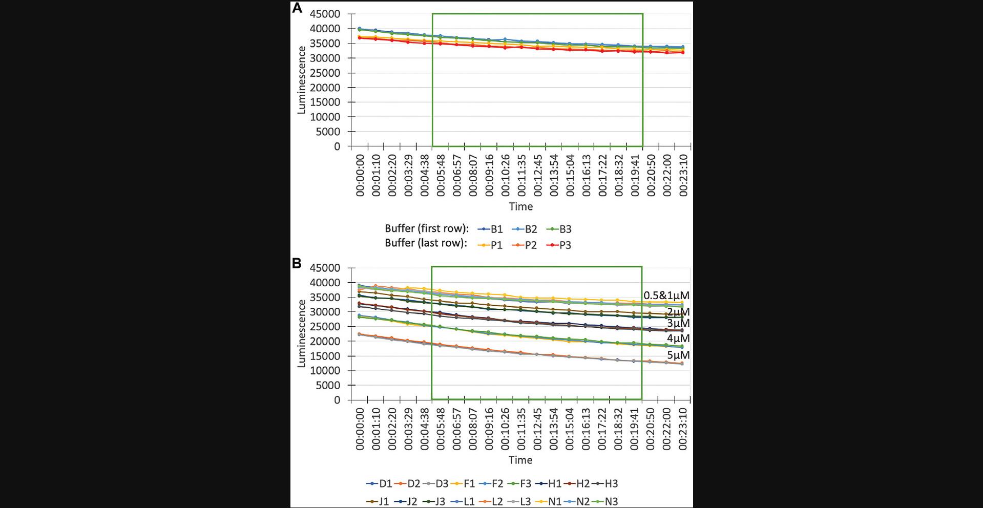
According to the assay manual, luminescence should be measured after 5 min. We average the luminescence values from 5-20 min for every assay in order to smooth out possible small deviations in the luminescence curve. As long as the time window begins after 5 min, the exact time window is less important than using the same time window for every assay.
The data from this assay can be used to compare the activity of different GTPases, the activity of two different effectors on a single GTPase, or the activity of one effector on different GTPases, as long as all samples are part of the same assay (to avoid small variability between assays) and are used at the same concentration.
GTPase cycling rates k1, k2. To increase comparability of GTPase and effector activities, we developed a GTPase cycling model (Supporting Information S8). Support Protocol 2 describes how the model can be used to fit data for Ras. In short, we fit an exponential to the amount of remaining GTP (Supporting Information S8) using Eqn. 1, where [Ras] is used for [GTPase]. Here, K refers to the overall GTP hydrolysis rate and depends on the concentration of Ras. GTPase cycling rates k describe the rate of the entire GTPase cycle of Ras. The model fits two cycling rates (k 1 and k 2) for every GTPase. K 1 accounts for the linear contribution of the GTPase (K 1 = k 1[GTPase]), while K 2 accounts for the quadratic contribution (K 2 = k 2[GTPase]2), which can be due to dimerization or other cooperative effects increasing the activity of the enzyme (for examples, see Zhang et al., 1999). The bigger the K 2/K 1 ratio, the bigger the contribution of the nonlinear term. This can suggest that the GTPase forms a dimer that is more active than the monomer, but additional studies examining GTPase di- and oligomerization are required before making such a deduction. The data indicate that some effect leads to a nonlinear concentration dependence of K , but does not reveal its origin. Ras does not show a linear concentration dependence (Fig. 8A) and is dominated by k 2 (Fig. 8B; k 2 >>> k 1). In this case, this is likely due to dimerization, as Ras GTPases are known to dimerize.
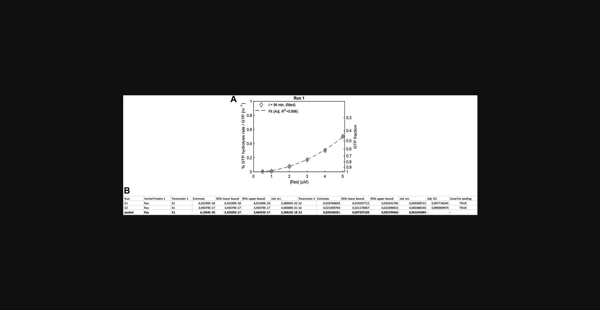
Output file structure and pooling of k rates. Estimates of Ras cycling rates k 1 and k 2 are summarized in Data_summary.xlsx (Fig. 8B). The file is structured in the following way: The Run column shows the assay number and is followed by two Varied Protein columns stating which proteins were varied in the assay. If the assay contains only one varied protein, the second column is empty (as for this example). Next, Parameter 1 is named along with its values, 95% upper and lower bounds, and standard error. The same is repeated if there are additional parameters (Parameter 2 is shown). The last column lists the adjusted R 2 of the fit and a Boolean (‘Used for pooling’) if the experiment is used for pooling. For each assay (i.e., each run: E1, E2), the rate value estimates are shown. Below, in the ‘pooled’ row, the pooled values of k estimates are listed (details on weighting of k for pooling and error propagation are provided in Supporting Information S11).
An experiment can be excluded from pooling if c corr or standard errors of k are out of range. Decision criteria are set before analyzing the data using two parameters (see Support Protocol 2): (1) conc_corr_bounds states the range of c corr that allows assays to be included in pooling, and (2) k_low_err_filt.Ras states if assays with low standard errors (1–10 or lower) on values are excluded from pooling. In Support Protocol 2 (example 1), we used
conc_corr_bounds = [0.5 1.5];
k_low_err_filt.Ras = false;
for analyzing Ras data. Although conc_corr_bounds states the range of c corr that allows assays to be included in the pooling, it does not influence pooling of k 1 and k 2, as c corr is only used for fitting k 3,X (Eqns. 2,3). We set k_low_err_filt.Ras to false so experiments with low standard errors on k values are not excluded from pooling. This makes sense for Ras, as Ras is dominated by k 2 and has k 1 ≈ 0 (and thus k 1 errors are close to 0).
Example 2
For this example, data are provided (spreadsheet: example2-matlab.xlsx in the Data folder; see Data Availability), for the following set of GTPase assays:
(A) Cdc42 (GTPase) dilutions (B) Cdc24 (GEF) dilutions using a constant Cdc42 concentration (C) Rga2 (GAP) dilutions using a constant Cdc42 concentration (D) Cdc24 and Rga2 dilutions using a constant Cdc42 concentration
The analysis is described in Support Protocol 2. In short, a GTPase cycling model (Supporting Information S8) is fitted using Eqn. 4. Here, K refers to the overall GTP hydrolysis rate and depends on the concentrations of Cdc42 and effectors Cdc24 and Rga2. First, the data for Cdc42 serial dilutions (group A) are fitted with an exponential to obtain estimates of GTPase cycling rates k 1 and k 2 for each experiment. These estimates are then bundled to get a single pooled estimate for k 1 and k 2. Next, Cdc42:Cdc24, Cdc42:Rga2, and Cdc42:Cdc24:Rga2 mixtures (groups B, C, and D) are fitted to obtain estimates for the correction factors c corr and cycling rates k 3 (measuring the impact of the effector on GTPase cycling) for every experiment. These latter estimates can then be pooled to obtain a single estimate for the k 3 values (a pooled estimate for c corr has no function here).
Correction factors ccorr. The correction factor c corr accounts for variability between assays, i.e., for the observation that the rates for the GTPase can vary between assays. Possible reasons for this include (1) small concentration differences introduced by pipetting of small volumes, (2) temperature and shaker speed fluctuations during incubation, (3) small changes in effective GTPase concentration through sequestration of GTPases in complexes with effectors, and/or (4) intrinsic changes in protein activities due to other external conditions. c corr maps all factors that lead to variations between assays onto the GTPase concentration. The correction factor is estimated for each experiment individually, relative to a predefined GTPase serial dilution assay. This is done by matching the overall hydrolysis rate at zero effector concentration inferred from the fit to the estimated overall hydrolysis rate based on the GTPase serial dilution assay. Concretely, c corr follows from:
where
To implement this recommendation, we used conc_corr_bounds = [0.5 1.5] for analyzing the data set in Support Protocol 2, example 1. This means that assays yielding c corr values <0.5 and >1.5 will be excluded from pooling. Figure 9 shows a histogram of all correction factors. Apart from one assay that yielded c corr ≈ 0.1, all c corr values were within range, with most values being close to 1.
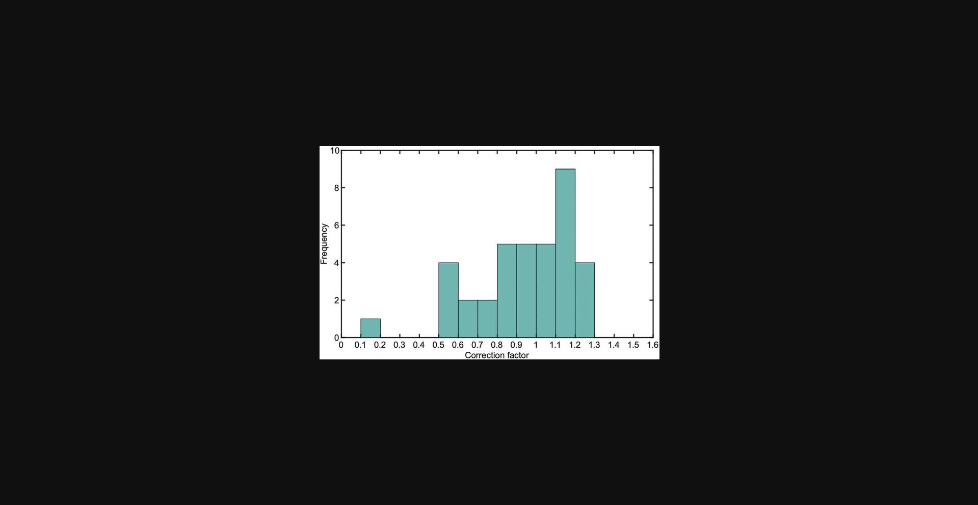
Data_summary.xlsx states correction factors as Parameter 1 for assays in which Cdc24 and/or Rga2 effectors are varied (Varied Proteins 1 and 2). Correction factor errors are discussed in Supporting Information S11.
GTPase cycling rates k3. GTPase cycling rates k describe the rate of the entire GTPase cycle of the GTPase or the effect of an effector on the overall rate. Cycling rates k 3,X can thus describe how strongly effector X affects the GTPase cycle, but do not reveal which step of the GTPase cycle the effector is acting upon, how strongly the effector is effecting this step, or if multiple steps are affected. To investigate these mechanisms, other GTPase assays need to be conducted (see Background Information).
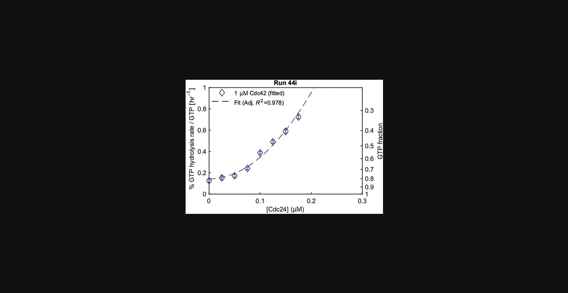
Assays of group B are used to fit cycling rates k 3,Cdc24, which describe the effect of Cdc24 on the overall GTPase cycle of Cdc42. We use a quadratic fit (K 3,Cdc24 = k 3,Cdc24[Cdc42][Cdc24]2) because the data show a nonlinear dependence of the overall rate K on Cdc24 concentration (Fig. 10). The fit is a phenomenological description of the data and does not reveal the origin of the nonlinearity. One possibility could be dimerization, with Cdc24 dimers exhibiting increased activity (Tschirpke, Daalman et al., 2023). Values of k 3,Cdc24 are shown in Data_summary.xlsx as Parameter 2 for assays in which Cdc24 is varied (Varied Protein 1). In a similar fashion, assays of group C are used to fit cycling rates k 3,Rga2, which describe the effect of Rga2 on the overall GTPase cycle rate of Cdc42. A linear fit (K 3,Rga2 = k 3,Rga2[Cdc42][Rga2]) was used to describe the data.
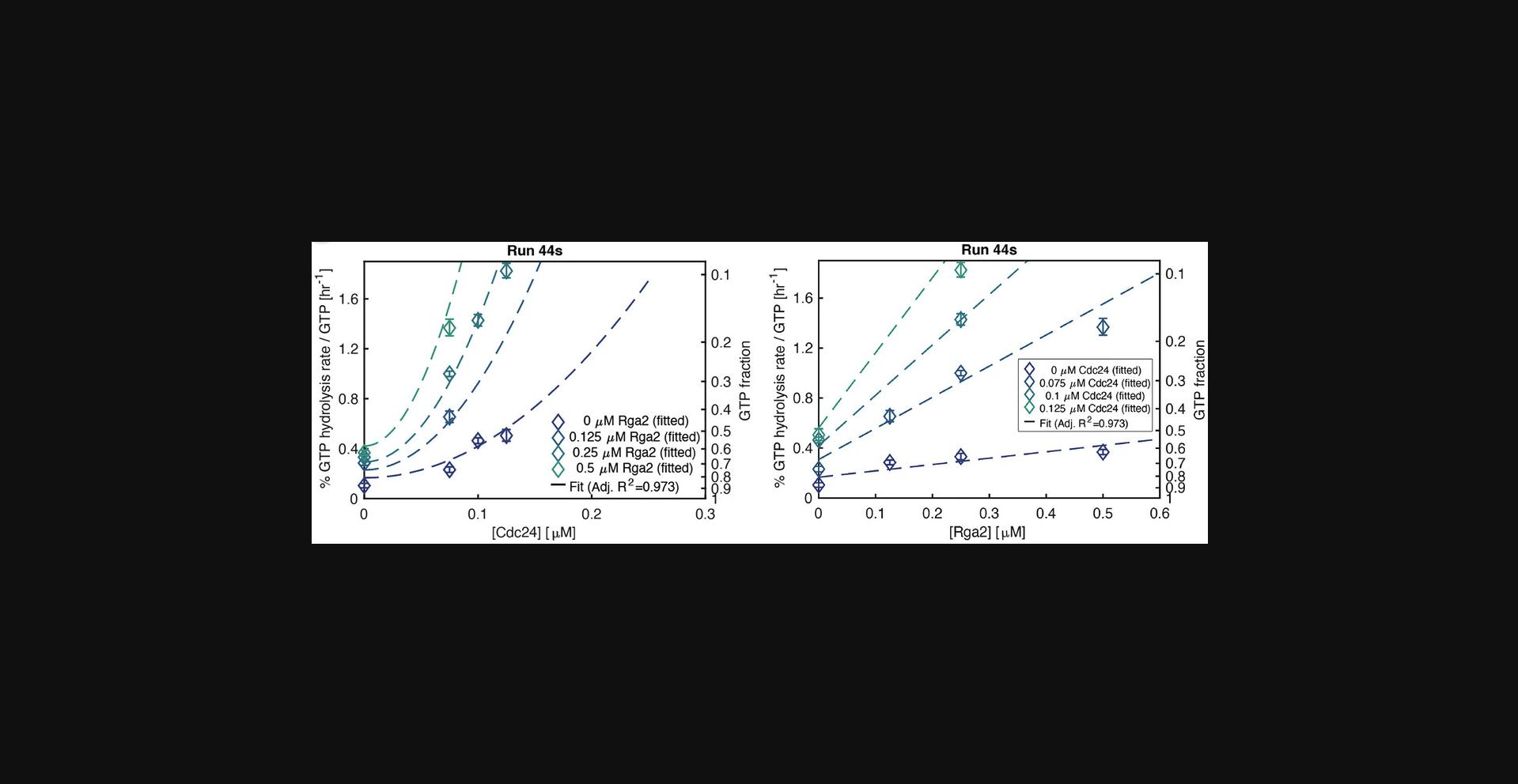
Data of group D contain mixtures of Cdc42:Cdc24, Cdc42:Rga2, and Cdc42:Cdc24:Rga2. Both Cdc24 and Rga2 are varied (Varied Protein 1 and 2). The data are fitted with three rate parameters (Fig. 11): k 3,Cdc24 (Parameter 2), k 3,Rga2 (Parameter 3), and k 3,Cdc24,Rga2 (Parameter 4). k 3,Cdc24 and k 3,Rga2 describe the effects of Cdc24 or Rga2 on the entire GTPase cycle. These rates should be close to those obtained in assays using only Cdc42:Cdc24 or Cdc42:Rga2 (Fig. 12). A large difference can indicate a problem with the fit or the assay. The cycling rate k 3,Cdc24,Rga2 accounts for any potential synergy between the two effectors. When k 3,Cdc24,Rga2 = 0, there is no interaction between the proteins. When k 3,Cdc24,Rga2 < 0, the proteins antagonize/inhibit each other, and when k 3,Cdc24,Rga2 > 0 there is synergy. Again, any interaction between the proteins refers to their combined effect on the overall rate. (The significance of the deviation from zero is also tested using Ruxton, 2006). The p value for the null hypothesis of zero interaction is stored in the Data_assays.mat output file, in the Assays_processed variable, in the field of that assay, in the subfield ’k_tot’, under ’Interaction_p’. While a positive k 3,Cdc24,Rga2 indicates that there is some synergy, it does not reveal the origin of the synergy. It could be due to physical protein-protein interactions or to rate-limiting steps in the cycle that are relieved when both proteins are added (Tschirpke, Daalman et al., 2023). One must thus be careful in interpretating this rate.
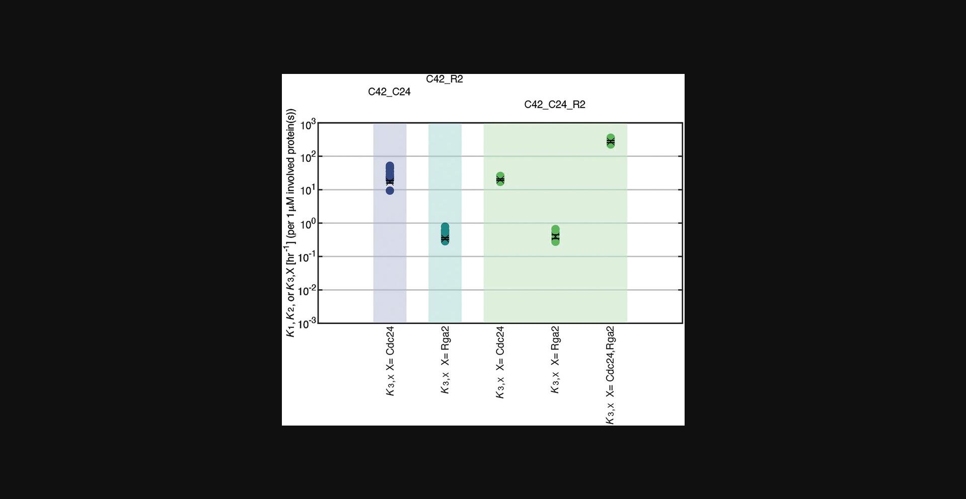
Comparison of cycling rates k. Overall GTP hydrolysis rates K are concentration dependent and have the unit hr−1. Cycling rates k are concentration-independent, but the different rates have different units (µM−1hr−1 for k 1, µM−2hr−1 for k 2, µM−3hr−1 for k 3,Cdc24, µM−2hr−1 for k 3,Rga2, and µM−4hr−1 for k 3,Cdc24,Rga2), making them difficult to compare. The easiest way to represent all rates in one plot is to plot overall GTP hydrolysis rates K for 1 µM of each protein (Fig. 12). However, one has to consider the different concentration dependencies when interpreting/comparing K rates. A rate that scales quadratically with protein concentration will be twice as big as a rate that scales linearly when the protein concentration is doubled. Some rates may also be valid only for the regime in which they were fitted in (e.g., they may show saturation in higher concentration regimes). Thus, one must consider which protein concentrations are used to calculate K in order to make cycling rates k comparable.
Time Considerations
GTPase assays usually take a few hours, some of which is consumed by incubation steps. For an assay involving eight samples (including six serial dilutions of GTPase) and using an incubation time of 1.5 hr, we estimate 30 min for preparation of materials and solutions, 2 hr for conducting the assay, and another 30 min for the luminescence readout. This amounts to a total of 3 hr, including 2 hr for incubation/measurement steps. Assays encompassing more samples may involve longer preparation times (as more protein dilutions need to be prepared). If proteins need to be dialyzed into a suitable buffer first, an additional dialysis step is required. The analysis time depends on the level of automatization and can range from a few minutes to 30-40 min. If the first step is done manually in a spreadsheet editor, ∼30 min are needed for this step. The subsequent analysis in Matlab requires only a few minutes of runtime.
Acknowledgments
We thank D. McCusker (University of Bordeaux) for plasmid pDM272 and N. Dekker (TU Delft) for plasmid pET28a-His-mcm10-Sortase-Flag. L. Laan gratefully acknowledges funding from the European Research Council under the European Union's Horizon 2020 Research and Innovation Programme (grant agreement 758132) and from the Netherlands Organization for Scientific Research (Nederlandse Organisatie voor Wetenschappelijk Onderzoek) through a Vidi grant (016.Vidi.171.060). S. Tschirpke gratefully acknowledges funding from the Kavli Synergy Post-doctoral Fellowship program of the Kavli Institute of Nanoscience Delft.
Author Contributions
Sophie Tschirpke : Conceptualization; formal analysis; investigation; methodology; project administration; validation; visualization; writing—original draft; writing—review and editing. Werner Daalman : Conceptualization; formal analysis; investigation; methodology; software; validation; writing—original draft; writing—review and editing. Liedewij Laan : Funding acquisition; project administration; supervision; writing—review and editing.
Conflict of Interest
The authors declare that they have no known competing financial interests or personal relationships that could have appeared to influence the work reported in this paper.
Open Research
Data Availability Statement
The data that support and exemplify the protocols are openly available at https://data.4tu.nl at http://doi.org/10.4121/ac196f25-1c20-4c0c-a0b9-f01cd3fadc45.
Supporting Information
| Filename | Description |
|---|---|
| cpz11000-sup-0001-SuppMat.pdf1.9 MB | Supporting Information S1. Preparation sheets for conducting GTPase assays with one, two, or three sample rows. Supporting Information S2. Prepared plate and preparatory sheet for a GTPase assay of six Ras GTPase serial dilutions (example 1). Supporting Information S3. Examples of how fluorescently labeled proteins affect the luminescence readout of GTPase assays. Supporting Information S4. Verification that the GTP concentration in GTPase assays declines exponentially with time. Supporting Information S5. Luminescence spill-over in directly neighboring plate wells. Supporting Information S6. Demonstration that 10 mM ADP can be reused, but 2× GTP solution cannot. Supporting Information S7. Luminescence values can vary between distinct detection reagent batches. Supporting Information S8. Brief description of the GTPase activity model used to determine GTPase cycling rates. Supporting Information S9. Description of the Python script used to reformat data in Support Protocol 1. Supporting Information S10. Description of plotting functions referred to in Support Protocol 2. Supporting Information S11. Extended description of the GTPase activity model used to determine GTPase cycling rates. |
Please note: The publisher is not responsible for the content or functionality of any supporting information supplied by the authors. Any queries (other than missing content) should be directed to the corresponding author for the article.
Literature Cited
- Bezeljak, U., Loya, H., Kaczmarek, B., Saunders, T. E., & Loose, M. (2020). Stochastic activation and bistability in a Rab GTPase regulatory network. Proceedings of the National Academy of Sciences of the United States of America , 117(12), 6540–6549. https://doi.org/10.1073/pnas.1921027117
- Bos, J., Rehmann, H., & Wittinghofer, A. (2009). GEFs and GAPs: Critical elements in the control of small G proteins. Cell , 16(3), 374–383. https://doi.org/10.1016/j.cell.2007.05.018
- Cherfils, J., & Zeghouf, M. (2013). Regulation of small GTPases by GEFs, GAPs, and GDIs. Physiological Reviews , 93(1), 269–309. https://doi.org/10.1152/physrev.00003.2012
- Kang, P. J., Béven, L., Hariharan, S., & Park, H. O. (2010). The Rsr1/Bud1 GTPase interacts with itself and the Cdc42 GTPase during bud-site selection and polarity establishment in budding yeast. Molecular Biology of the Cell , 21(17), 3007–3016. https://doi.org/10.1091/mbc.e10-03-0232
- Kohyama, S., Merino-Salomón, A., & Schwille, P. (2022). In vitro assembly, positioning and contraction of a division ring in minimal cells. Nature Communications , 13(1), 6098. https://doi.org/10.1038/s41467-022-33679-x
- Loose, M., Fischer-Friedrich, E., Ries, J., Kruse, K., & Schwille, P. (2008). Spatial regulators for bacterial cell division self-organize into surface waves in vitro. Science , 320(5877), 789–792. https://doi.org/10.1126/science.1154413
- Rapali, P., Mitteau, R., Braun, C., Massoni-Laporte, A., Ünlü, C., Bataille, L., Arramon, F. S., Gygi, S. P., & McCusker, D. (2017). Scaffold-mediated gating of Cdc42 signalling flux. eLife , 6, 1–18. https://doi.org/10.7554/eLife.25257
- Ruxton, G. D. (2006). The unequal variance t-test is an underused alternative to Student's t-test and the Mann-Whitney U test. Behavioral Ecology , 17(4), 688–690. https://doi.org/10.1093/beheco/ark016
- Smith, N. J., van der Walt, S., & Firing, E. (2015). Magma, inferno, plasma and viridis colormaps. https://github.com/bids/colormap
- Tschirpke, S., Daalman, W., & Laan, L. (2023). The GEF Cdc24 and GAP Rga2 synergistically regulate Cdc42 GTPase cycling. BioRxiv , https://doi.org/10.1101/2023.06.26.546500
- Tschirpke, S., van Opstal, F., van der Valk, R., Daalman, W. K.-G., & Laan, L. (2023). A guide to the in vitro reconstitution of Cdc42 activity and its regulation. BioRxiv , https://doi.org/10.1101/2023.04.24.538075
- Vendel, K. J. A., Tschirpke, S., Shamsi, F., Dogterom, M., & Laan, L. (2019). Minimal in vitro systems shed light on cell polarity. Journal of Cell Science , 132(4), 1–21. https://doi.org/10.1242/jcs.217554
- Vetter, I. R., & Wittinghofer, A. (2001). The guanine nucleotide-binding switch in three dimensions. Science , 294(5545), 1299–1304. https://doi.org/10.1126/science.1062023
- Zhang, B., Gao, Y., Moon, S. Y., Zhang, Y., & Zheng, Y. (2001). Oligomerization of Rac1 GTPase mediated by the carboxyl-terminal polybasic domain. Journal of Biological Chemistry , 276(12), 8958–8967. https://doi.org/10.1074/jbc.M008720200
- Zhang, B., Wang, Z. X., & Zheng, Y. (1997). Characterization of the interactions between the small GTPase Cdc42 and its GTPase-activating proteins and putative effectors: Comparison of kinetic properties of Cdc42 binding to the Cdc42-interactive domains. Journal of Biological Chemistry , 272(35), 21999–22007. https://doi.org/10.1074/jbc.272.35.21999
- Zhang, B., Zhang, Y., Collins, C. C., Johnson, D. I., & Zheng, Y. (1999). A built-in arginine finger triggers the self-stimulatory GTPase-activating activity of Rho family GTPases. Journal of Biological Chemistry , 274(5), 2609–2612. https://doi.org/10.1074/jbc.274.5.2609
- Zhang, B., & Zheng, Y. (1998). Negative regulation of Rho family GTPases Cdc42 and Rac2 by homodimer formation. Journal of Biological Chemistry , 273(40), 25728–25733. https://doi.org/10.1074/jbc.273.40.25728

