Mouse Brain Heatmap - Whole brain data compilation and quality control

Begin by hitting the browse button labeled for the ‘ left side ’ and select all files in the ‘left’ folder.

If you have a ‘data’ folder, select all files in that folder instead.

Hit the ‘open’ button to start loading the data.

While that is loading you can hit the browse button labeled for the ‘ right side ’ and select the files in the ‘right’ folder and hit the ‘open’ button to begin loading that data.

Wait until there is a message on the right side of the app that says the last side you loaded is done.

Double check that the above step has appeared and then click the button labeled ‘ click this when all files are done loading ’.

Wait until the message on the right side changes and mentions the ‘blank annotation’ and the ‘checkpoint’ are done.

Press the button labeled ‘ Download Checkpoint 1 ’ and save it within your project folder. This will be used the next time you load the data.

Press the button labeled ‘ Download blank annotation file ’ and save it within your project folder.

Open your file explorer and navigate to your project folder.

Open the annotation file you just downloaded and fill out all columns labeled with “NA” (if you don’t have a column, then you may leave it NA)

A	B
Mouse	Mouse name
Sex	Mouse sex
Treatment	Mouse treatment type
MPI	Months post injection
Genotype	Mouse genotype
Marker	What you are comparing in the mice, such as a cell type or strain.
Include	Use this column if you wish to subset the full dataset.
	Y = include
	N = do not include

Save this file as a CSV file with a different name so that you know you have completed it.

Reload the webpage or stop and restart the RStudio app.

Begin by clicking the Browse button labeled by the phrase ‘ Input checkpoint 1 here ’ and select “checkpoint1.rds” you saved earlier and click ‘open’.

Check the right side of the screen for confirmation that the checkpoint is done loading and then click the browse button to input in the annotation file you finished creating.

Once that has completed (check the right side for text saying has finished), download Checkpoint 2 somewhere you have easy access to

Once that is complete you may notice that the box labeled for selecting your ‘ x axis variables ’ now has options to choose from. Please note the following when you select these variables:

Next, select the ‘ y axis variables ’ and note the following when selecting them:

Select the ‘ display’ y axis variables next noting the following:

When you have selected variables for all the above options, click the button labeled ‘ Get Options ’.

Next, look at all the options that are selected in the box labeled with ‘ variables to see ’ and confirm you want to see all of the above variables on the heatmap.

This step will determine the values of the heatmap, so pay close attention : From the dropdown list labeled ‘ select the nutil variable ’, select the variable you will be using as your value (i.e. Load)

If you would like to change the variable in any way:

Select Multiply by 100 if you would like to do as stated.

Select Use variables if you would like to select variables to create a percentage . Select the variables based on the following information:

• Segments by each variable labeled here and then creates percentages of any other variable you selected above that is not in this box.
• Here the program will group your data based on your selections and create a percentage separating from the largest to the smallest designation. For example:

1. If your rows were ‘mouse’ and ‘marker’ (marker has two options per mouse), your selected nutil variable was ‘object count’, and you selected, ‘Mouse’, ‘side’, and ‘daughter’ here; it would first separate the data by mouse, then by side, then by daughter. Then it would look at the designations of the row and see that it’s separated by mouse and marker so it calculates the percent each marker takes up as it is already segmented by mouse.

• If you are hoping to compare the percentage of elements in a variable (such as ‘pSyn+’ to ‘pSyn-‘ in the variable ‘marker’), then do not include that variable in this segmentation as it would then turn out to be 100% for each of them
• Common Examples :

1. ‘side’, ‘mouse’, and ‘daughter’
2. ‘mouse’, ‘daughter’

If you would like the data to be in log 10 scale : check the corresponding box.

If you would like your heatmap to be trimmed : check the corresponding box. (This does not affect the calculations.)

If you would like to remove ABA regions from your heatmap, select any amount of them from the drop down labeled ‘ Select any regions to remove ’.

If you would like row and column names : select from the corresponding drop down boxes and select what you would like to see.

The color scale is not something you will need to adjust your first time loading the heatmap.

Now that you are done selecting the base variables for your heatmap, click the button labeled ‘ Create heatmap ’ and wait for a preview to appear in the right side.

Now that the heatmap is done, you will note some text at the top of the right side which says ‘min’ and ‘max’. Please enter these values into the textboxes labeled ‘ Min Value ’ and ‘ Max Value ’ for the color scale .

At this point, you can adjust the options under the label ‘ Custom Colors ’. If you would like to , then select either the Viridis color scale checkbox, the 2 color scale checkbox, or the 3 color scale box , and then choose or adjust the colors to what you would like.

When you are done, click the ‘ create heatmap ’ button again and wait for the preview to appear.

To save the heatmap : you have two options you can choose from or download both.

• Click the button labeled ‘ Download full Heatmap ’ and this will download a heatmap with all the information you selected above. Make sure to download it into a directory you can easily access to check if you like your chosen options.
• Click the button labeled ‘ Download Just the Plot ’ and this will download a heatmap without any of the legends for easy editing. Make sure to download it into a directory you can easily access to check if you like your chosen options.

Look at your heatmap and determine if you need to change anything . If you do, start from step 3 and check over each step at a time.

Begin by clicking the Browse button labeled by the phrase ‘ Input checkpoint 2 here ’ and select “checkpoint2.rds” you saved earlier and click ‘open’.

Check the right side of the screen for confirmation that the checkpoint is done loading and then continue from step 4 above .

If you would like to display data in anatomical space, take it into the MBH app , click the ‘ Download MBH Table ’ button and save it wherever you can access it.

If you would like the color scheme to also be the same in the MBH app , click the ‘ Download Colors ’ button.

If you would like the values of the heatmap or any of the axis annotation information of the heatmap, click the buttons labeled ‘ Download Data ’, ‘ Download AnnoX ’, and ‘ Download AnnoY '.

Finally, if you would like access to the many variables created during this program running or the data frame that contains the raw data at any point:

Open the app in R Studio.

To save a variable as a csv file write the following code in the console:

• .write.csv(variableName, “filename.csv”)
• If you would like to designate the location of the file , include the file path in front of the filename with all back slashes replaced with forward slashes

1. “~\projects\file.csv” is incorrect
2. “~/projects/file.csv” is correct

Run through all of the steps.

Once it has created a heatmap, wait a minute or two for everything to fully load.

Click back into R Studio without closing the app.

Find the console in the bottom left corner and click the button that looks like a stop sign ONCE and only once.

Wait very patiently for the app to close on its own.

If it gives you an error like below click ‘No’ and wait some more.

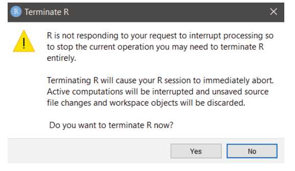
Eventually it will stop the app and variables will appear in the top right box labeled ‘environment’.

To see these variables, double click their names to open a viewer pane.

Determine whether you want to plot single or multi-figure plots. Upload your compiled matrix by hitting browse on the prompt ‘ Please upload the MBH table output ’.

• This should be labeled as ‘MBHTable’ and is generated after selecting ‘Download MBH table’ in the N2U program.
• In theory, any csv file following the same format as seen in the MBH table would suffice for this workflow.

If you generated a custom color scheme in the N2U app, upload the .rds file in the browse button under the ‘If desired, upload heatmapColors.rds here’ (not a necessary step if using the default scheme).

Select the Figure Number corresponding to the sections for your project.

This will only be one Figure Number if creating single-figure plots. Multi-figure Numbers should be separated by a comma without spaces between them.

If you are unsure which figure you are working with, visit the ABA website and determine which section (out of 132) corresponds to the anatomical region(s) you are interested in plotting.

Select the measure summary you would like to have plotted.

Select the depth level for atlas regions.

The remaining dropdowns allow you to choose what you would like to plot.

Single-fig allows you to compare across conditions

1. The MPI, genotype, treatments, and markers can be selected for when plotting. The data for mice within the conditions set here will be summarized and displayed in plots.
2. By default, plots for each sex will be distinguished. If you would like to combine summary results across sexes, select ‘Averaged’ in the dropdown box under ‘Sexes to Plot’.

Multi-fig will only allow you to plot for a single condition

1. Whereas single-fig can generate multiple plots for each condition in the same output, multi-fig only displays a single condition at a time.

Select ‘Plot data’ to create the heatmaps you have set. This may take time to load. Each time you adjust conditions or inputs you will need to reselect ‘Plot data’ to see the new plots.

‘Download Plot’ generates .svg files for generated plots.

‘Download Data’ generates a .csv with information on what anatomical regions are plotting and the values being displayed in each.