Leveraging AI Advances and Online Tools for Structure-Based Variant Analysis
Francisco J. Guzmán-Vega, Francisco J. Guzmán-Vega, Ana C. González-Álvarez, Ana C. González-Álvarez, Karla A. Peña-Guerra, Karla A. Peña-Guerra, Kelly J. Cardona-Londoño, Kelly J. Cardona-Londoño, Stefan T. Arold, Stefan T. Arold
Abstract
Understanding how a gene variant affects protein function is important in life science, as it helps explain traits or dysfunctions in organisms. In a clinical setting, this understanding makes it possible to improve and personalize patient care. Bioinformatic tools often only assign a pathogenicity score, rather than providing information about the molecular basis for phenotypes. Experimental testing can furnish this information, but this is slow and costly and requires expertise and equipment not available in a clinical setting. Conversely, mapping a gene variant onto the three-dimensional (3D) protein structure provides a fast molecular assessment free of charge. Before 2021, this type of analysis was severely limited by the availability of experimentally determined 3D protein structures. Advances in artificial intelligence algorithms now allow confident prediction of protein structural features from sequence alone. The aim of the protocols presented here is to enable non-experts to use databases and online tools to investigate the molecular effect of a genetic variant. The Basic Protocol relies only on the online resources AlphaFold, Protein Structure Database, and UniProt. Alternate Protocols document the usage of the Protein Data Bank, SWISS-MODEL, ColabFold, and PyMOL for structure-based variant analysis. © 2023 The Authors. Current Protocols published by Wiley Periodicals LLC.
Basic Protocol : 3D Mapping based on UniProt and AlphaFold
Alternate Protocol 1 : Using experimental models from the PDB
Alternate Protocol 2 : Using information from homology modeling with SWISS-MODEL
Alternate Protocol 3 : Predicting 3D structures with ColabFold
Alternate Protocol 4 : Structure visualization and analysis with PyMOL
INTRODUCTION
Genetic variations can result in both advantageous adaptations and detrimental diseases. Many changes that have an effect on an individual's phenotype are located in the protein-coding regions of genomes (Backman et al., 2021). Hence, understanding how a gene variant affects its protein product is crucial for comprehending both normal and abnormal biological processes. In medicine, this knowledge can facilitate personalized treatments based on an individual's genetic profile, leading to improved diagnoses, more effective treatments, reduced side effects, and better health outcomes. Despite significant progress made in linking specific genes to certain disorders, determining the variants and underlying biological mechanisms remains a challenge for many disease phenotypes. Consequently, cancer drivers may not be identified in time, and many patients with suspected rare genetic diseases either never receive a definitive diagnosis or do so only after a lengthy and exhausting “diagnostic odyssey,” during which they may experience irreversible damage (MacArthur et al., 2014).
Traditional methods for predicting variant pathogenicity typically employ various classification algorithms to generate a score indicating the likelihood of a variant being damaging. Among the most widely used in silico prediction tools are SIFT (Ng & Henikoff, 2001), PolyPhen-2 (Adzhubei et al., 2010, 2013), and CADD (Rentzsch et al., 2018). More recent methods utilize advanced deep-learning techniques (Frazer et al., 2021; Qi et al., 2021), including large language models (Brandes et al., 2022; Lin et al., 2023), to predict the pathogenicity of missense variants with greater accuracy. However, although predicted pathogenicity scores may aid in identifying a driver mutation, they do not elucidate how a variant impacts protein function.
A protein's function is dependent on its three-dimensional (3D) structural features. Several computational resources have been developed to predict or document the impact of amino acid substitutions on protein structures. For instance, Missense3D (Ittisoponpisan et al., 2019) predicts the structural damage resulting from a point mutation, and its associated Missense3D-BD database contains pre-calculated results for about 4 million known missense variants from the Humsavar, ClinVar, and gnomAD resources. VarSite (Laskowski et al., 2020) annotates known disease-associated variants in human genes with structural information derived from experimentally determined 3D structures in the Protein Data Bank (PDB). Although these resources are valuable for understanding the effects of mutations, they have limitations. Most notably, Missense3D-BD and VarSite only provide structural annotations for previously reported variants, and VarSite only annotates protein structures from the PDB, which contains (partial) structures of just 17% of human genes. Additionally, these tools currently lack important features for assessing the impact of a variant, such as information about proximity to protein sites involved in catalytic activity, regulation, or ligand binding. Finally, interpreting the features provided by Missense3D may be challenging without interactively visualizing the 3D structural context.
For these reasons, being able to view and study a novel mutated residue within its 3D structural context can be essential for understanding the causes and mechanisms of a disease. Before 2021, the ability to map an amino acid variant onto a 3D structure was severely limited due to the lack of reliable 3D structural information for more than 80% of human proteins. Homology modeling may infer the 3D structure of a human protein from known structures of similar nonhuman proteins, but the accuracy depends on the availability and sequence identity of structural templates.
In 2020, the AI-based method AlphaFold demonstrated its ability to predict the 3D structure of proteins from their amino acid sequence with an accuracy that can be on par with that of high-quality experimental structures (Jumper et al., 2021). In June 2021, AlphaFold became publicly available, and its Protein Structure Database now contains precalculated 3D structures for 200 million proteins, including all human proteins (Tunyasuvunakool et al., 2021; Varadi et al., 2021). This resource enables scientists and healthcare providers to quickly assess the impact of human gene variants. However, a step-by-step guide for structure-based variant analysis using these methods and resources is still needed.
We provide protocols to help non-experts, including clinicians and healthcare personnel, use these resources to quickly assess the molecular impact of a gene variant. The basic protocol relies only on online resources and allows non-experts to develop hypotheses about how a mutation affects protein function. Depending on the variant and protein, the information can be obtained within minutes to hours. Alternate protocols describe the use of additional programs and resources.
Understanding how a mutation affects a protein's structure and function is essential for linking phenotypes to gene variants and personalizing therapy. However, our protocol can be used to investigate the impact of mutations on any protein, including those from plants or bacteria.
STRATEGIC PLANNING
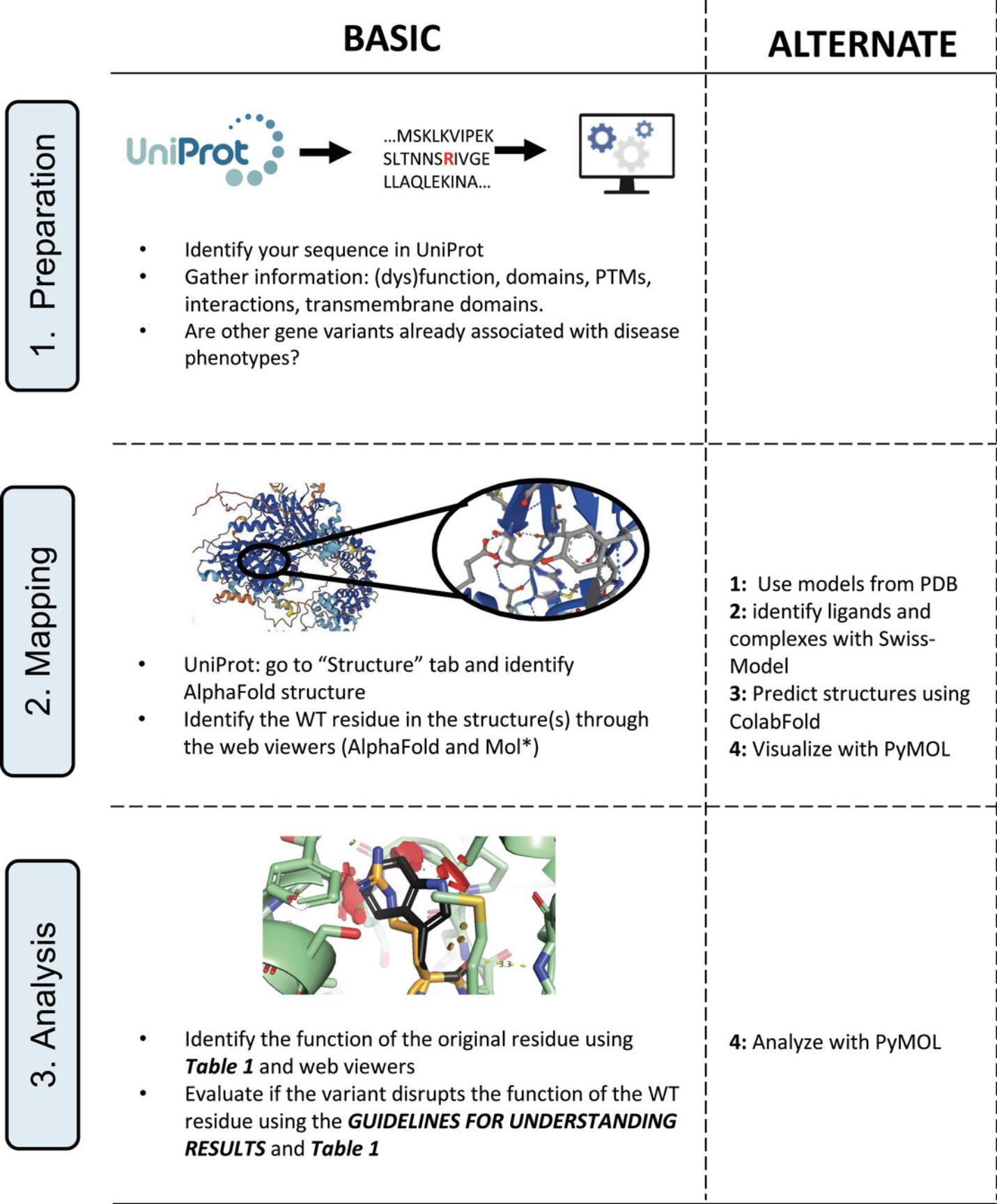
The Basic Protocol is the simplest approach, relying only on web-based tools. It uses information from the UniProt and AlphaFold databases and their online visualization tools. The protocol has three steps: Preparation, Mapping, and Analysis (Fig. 1). We also propose four Alternate Protocols for obtaining additional information Alternate Protocol 1 (Using experimental models from the PDB) and Alternate Protocol 2 (Using information from homology modeling with SWISS-MODEL) provide information on ligand binding or protein-protein interactions. Alternate Protocol 3 (Predicting 3D structures with ColabFold) produces 3D models of protein sequences not precalculated, such as specific truncations, isoforms, or protein complexes. Alternate Protocol 4 (Structure visualization and analysis with PyMOL) provides a focused protocol for the visualization and analysis of variants in 3D protein structures.
NOTE : All protocols involving animals must be reviewed and approved by the appropriate Animal Care and Use Committee and must follow regulations for the care and use of laboratory animals. Appropriate informed consent is necessary for obtaining and use of human study material.
Basic Protocol: 3D MAPPING BASED ON UniProt AND AlphaFold
The Basic Protocol is ideal for quickly evaluating standard protein forms precalculated by AlphaFold. The insights gained allow to identify, or rule out, effects linked to protein stability, and, in some cases, catalysis. If this protocol fails to yield conclusive results, we recommend the Alternate Protocols. As case examples for the Basic Protocol, we will analyze two protein variants (Arg799Cys and Arg918Trp) of the AGTPBP1 protein, implicated in infantile-onset neurodegeneration (Shashi et al., 2018).
Necessary Resources
Hardware
- Computer with internet access
Software
- Standard internet browser
Preparation
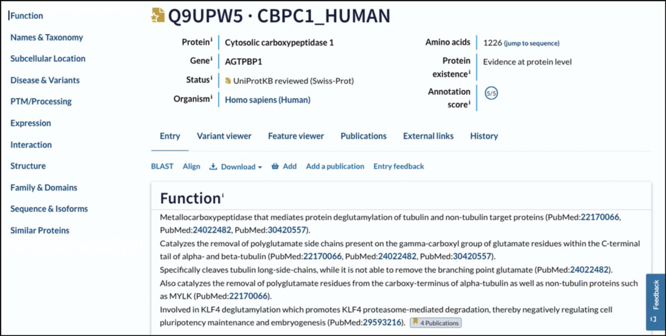
1.To identify the protein sequence of interest in UniProt, go to the UniProt website (https://www.uniprot.org/) and search for the name of its gene or transcript ID. Click on the entry for the correct species to access the entry website (Fig. 2).
2.In the entry page for your protein, click on “Sequence & Isoforms” in the section menu displayed at top left in the UniProt window (Fig. 3).
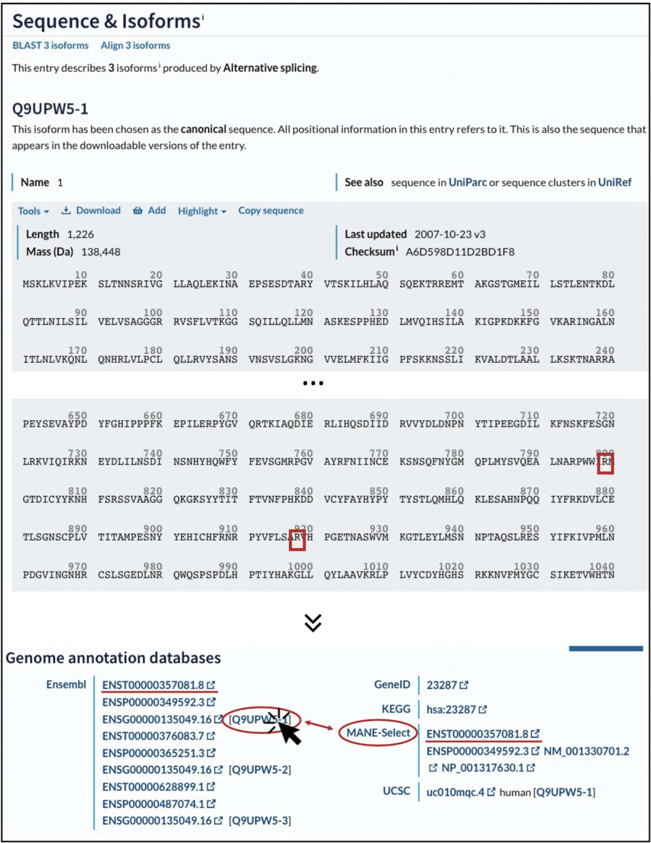
3.Verify that the chosen UniProt sequence contains the wild-type residue(s) at the correct position(s).
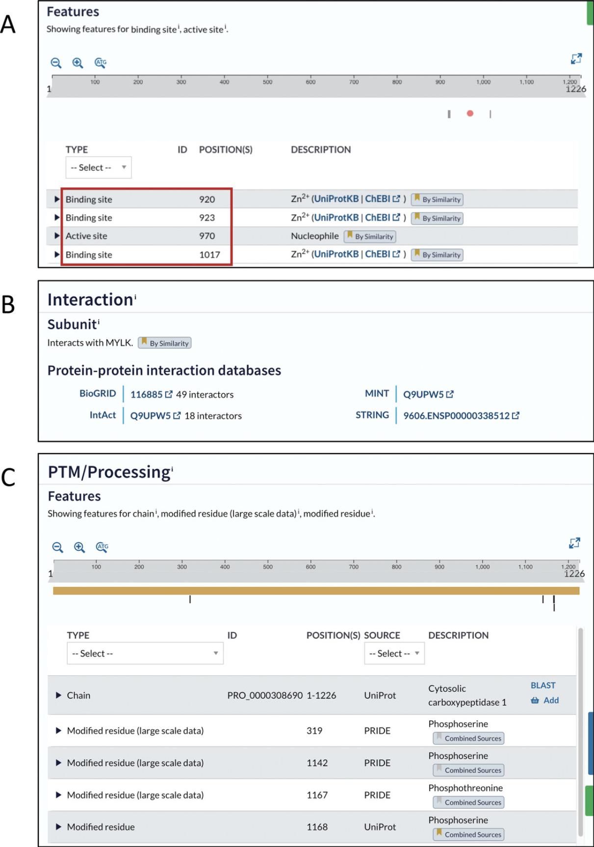
4.Gather general information on the gene from UniProt.
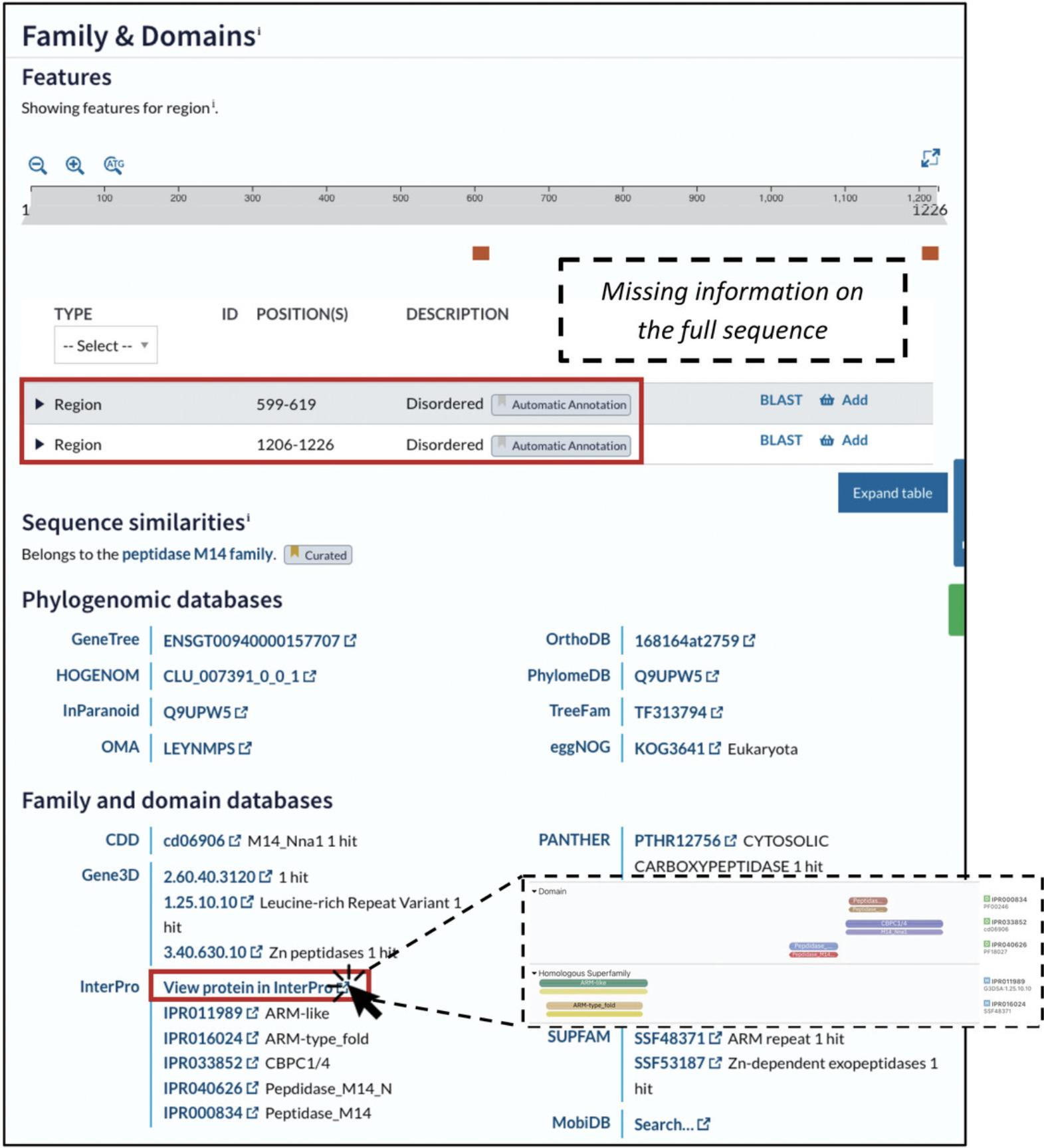
Mapping
After completing the preparation step, in which you identify the wild-type residue in the protein sequence and gather background information on the protein's function and features, the next step is mapping. In this step you will identify the wild-type residue of your variant in its 3D protein context. Below we describe the simplest way to do this by using pre-calculated AlphaFold structures and web-based visualization tools. Alternatively, you can obtain 3D structures from the PDB or through homology modeling and use other programs for structure visualization. These approaches are described in detail in Alternate Protocols 1-4.
5.To access AlphaFold structures on UniProt, scroll to the “Structure” section (Fig. 6). Below the interactive structure viewer, you will find a table with the available 3D structures for your protein.
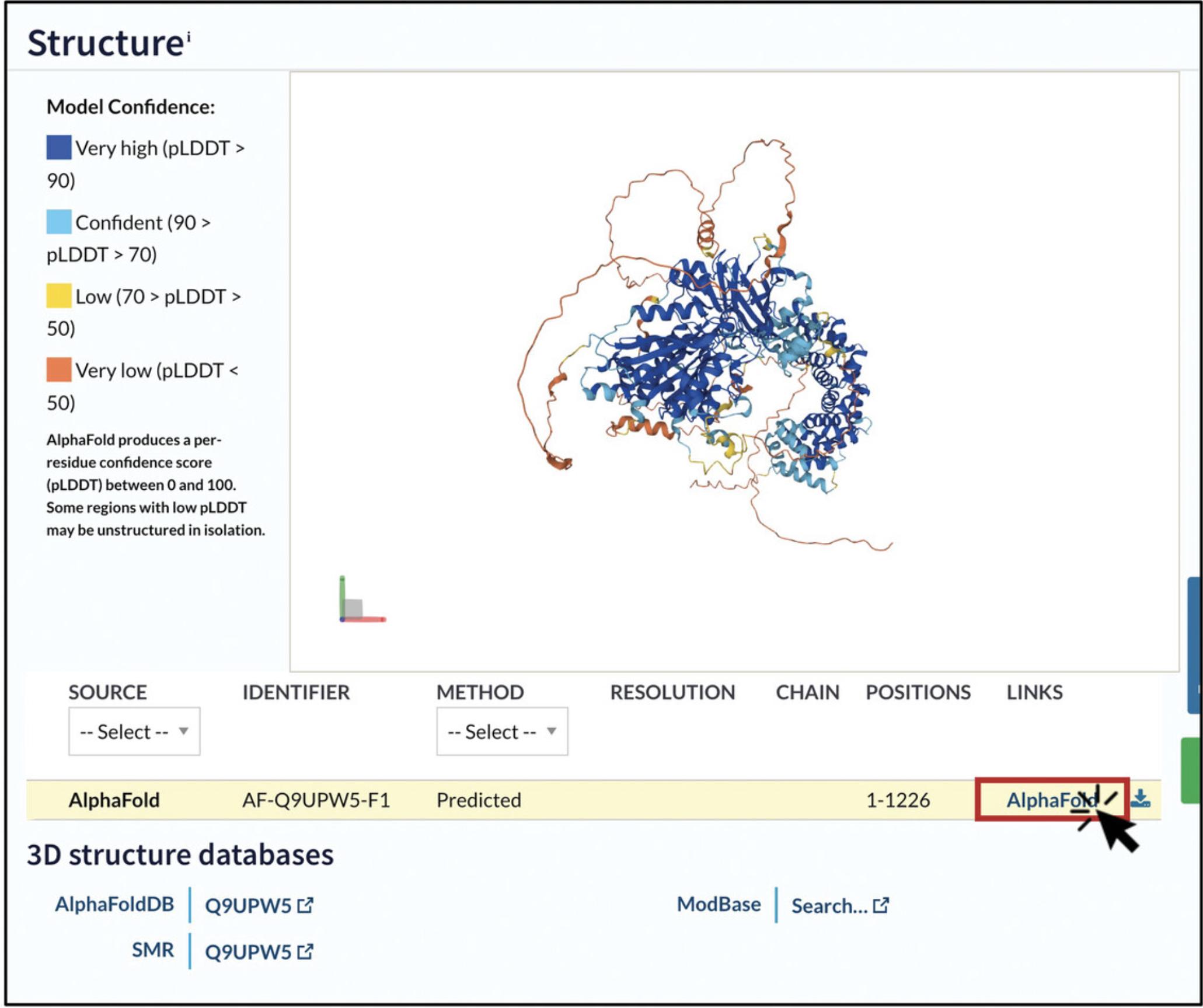
6.Look for the entry with “AlphaFold” in the “SOURCE” column and click on the hyperlink in the “LINKS” column. This will take you to the entry page for this model in the AlphaFold Protein Structure Database (https://alphafold.ebi.ac.uk/).
7.Map your residue onto the 3D structure by using the interactive AlphaFold Structure Viewer.
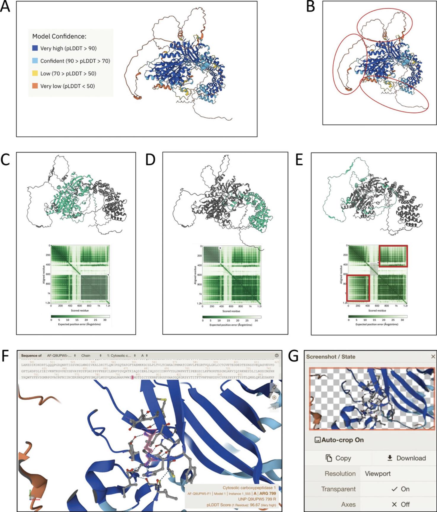
8.Assess the confidence in the relative positioning of residues and domains with the PAE plot.
9.Identify the wild-type residue in the 3D structure.
10.Click on a residue in the AlphaFold Structure or Sequence Viewer to get a zoomed-in view of the amino acid and its intramolecular interactions.
11.Capture and save an image of the visualization. In the top right corner of the Structure Viewer , there are three icons representing the following options: Top, to reset the view to the default settings; middle, to capture a screenshot of the current structure view (this can be copied or downloaded as a PNG file, with a transparent or white background; Fig. 7G); and bottom, to enable widescreen mode for a larger view of the model. Mouse over the icons to display their functions.
12.Assess whether the location of the residues of interest in the 3D model overlaps with a known functional feature.
13.Download the PDB model for further analysis. The AlphaFold model can be downloaded in the PDB file format to your local computer (“Download” > “PDB file”) and then be visualized with more versatile structure viewers, such as the PDB Mol* viewer (see Alternate Protocol 1, step 5) or PyMOL (see Alternate Protocol 4).
Analysis
14.Assess the function of the wild-type residue in its 3D context.
15.Assess the effect of the substitution on the 3D structure. The final step in analyzing the effect of a variant is to determine whether the substituting residue can maintain the function of the wild-type residue. Although the AlphaFold Structure Viewer does not allow substitution of the wild-type with the mutant residues in the display, the severity of a substitution can often be estimated by comparing the size and stereochemistry of the wild-type and mutant residues (see Table 1).
| Side chain | Amino acid | Size | Other | ||
|---|---|---|---|---|---|
| Negative | Aspartic acid | Asp | D | Medium large | Charged carboxylic acid group; often caps α-helices |
| Glutamic acid | Glu | E | Large, flexible | Charged moiety as in Asp, but longer carbon side chain | |
| Positive | Arginine | Arg | R | Large, flexible | Charged guanidino group; can coordinate phosphate groups |
| Lysine | Lys | K | Large, flexible | PTM of charged amine group is a major signal in epigenetics | |
| Histidine | His | H | Large | Aromatic imidazole group is partially protonated at physiological pH | |
| Uncharged polar | Asparagine | Asn | N | Medium large | Like Asp, but with polar carboxamide |
| Glutamine | Gln | Q | Large | Likes Glu, but with polar carboxamide | |
| Serine | Ser | S | Small | Small; can be phosphorylated | |
| Threonine | Thr | T | Medium-small | Like Ser but with additional hydrophobic moiety; can be phosphorylated | |
| Tyrosine | Tyr | Y | Large | Aromatic, with hydroxy moiety that can be phosphorylated or form H-bond | |
| Nonpolar | Alanine | Ala | A | Small | Rigid and small |
| Glycine | Gly | G | Tiny | No side chain; flexible; can form sharp turns in backbone | |
| Valine | Val | V | Medium-small | Larger than Ala, but smaller than Ile or Leu | |
| Leucine | Leu | L | Medium | Can often be replaced by Ile | |
| Isoleucine | Ile | I | Medium | Can often be replaced by Leu | |
| Proline | Pro | P | Small | Rigidifies backbone; breaks α-helices and β-strands | |
| Phenylalanine | Phe | F | Large | Aromatic; Tyr without hydroxy substituent | |
| Methionine | Met | M | Medium | Long, thin, and flexible | |
| Tryptophan | Trp | W | Large | Aromatic indole moiety that can also make a H-bond | |
| Cysteine | Cys | C | Small | Can form disulfide bonds | |
-
Note that all residues except Ile, Leu, and Phe can be subject to PTMs. Only charged residues can form ionic bonds (also called salt bridges); charged and uncharged polar residues can form hydrogen bonds (H-bonds). Of the nonpolar residues, only tryptophan can form an H-bond.
16.Next steps : This Basic Protocol, in conjunction with Table 1, provides a straightforward approach to evaluating the structural impact of variants at the molecular level. The AlphaFold Structure Viewer is also useful for creating figures for presentations and publications. However, precalculated AlphaFold models do not include ligands or cofactors. The AlphaFill server (https://alphafill.eu) attempts to automatically add ligands to precalculated AlphaFold structures based on experimental data. For example, the server correctly identifies the substrate-binding site for AGTPBP1 (Q9UPW5) using 25% identity but incorrectly suggests another ligand. Additionally, many proteins form multimers or are part of macromolecular complexes with other proteins or nucleic acids, which may be important for comprehensive variant analysis. Alternate Protocols 1, 2, and 3 provide guidance on accessing this information. Alternate Protocol 4 outlines simple steps for using PyMOL as a more versatile alternative to the online AlphaFold Structure Viewer for displaying and analyzing structures.
Alternate Protocol 1: USING EXPERIMENTAL MODELS FROM THE PDB
Precalculated AlphaFold models do not include cofactors or macromolecular binding partners and present only a single conformation, even though many proteins alternate between multiple structural states. If experimentally determined 3D structures of the affected protein are available, they may provide additional information. These experimental structures are freely accessible in the Protein Data Bank (PDB; https://rcsb.org). If no experimental structures have been reported for the gene region of interest, you can try using the SWISS-MODEL service described in Alternate Protocol 2.
As an example, we will evaluate the mutation Arg1748Cys in the gene SETD1B (Weerts et al., 2021).
Necessary Resources
Hardware
- Computer with internet access
Software
- Standard internet browser
Preparation
1.Go to the UniProt page for the human SETD1B gene (UniProt ID Q9UPS6; https://www.uniprot.org/uniprotkb/Q9UPS6/entry).
2.Scroll down to the “Sequence & Isoform” section and find the correct isoform for your analysis.
3.Gather functional information on the gene from UniProt.
Mapping
4.Click on the “Structure” section in the left-hand menu. In addition to the AlphaFold model, two experimentally solved structures are available for this protein, annotated as “PDB” in the “SOURCE” column of the Table.
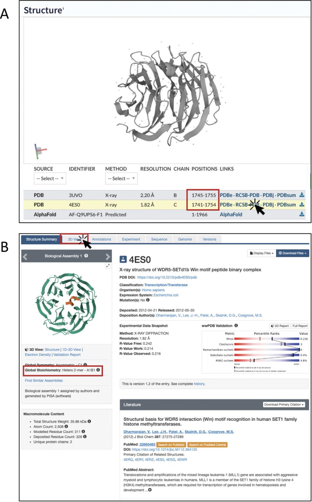
5.Click on the RCSB-PDB link in the “LINKS” column to be taken to the corresponding entry on the PDB website (Fig. 8B).
6.To interactively visualize the 3D structure with the PDB Mol* viewer, click on the 3D View tab at the top (Fig. 9A).
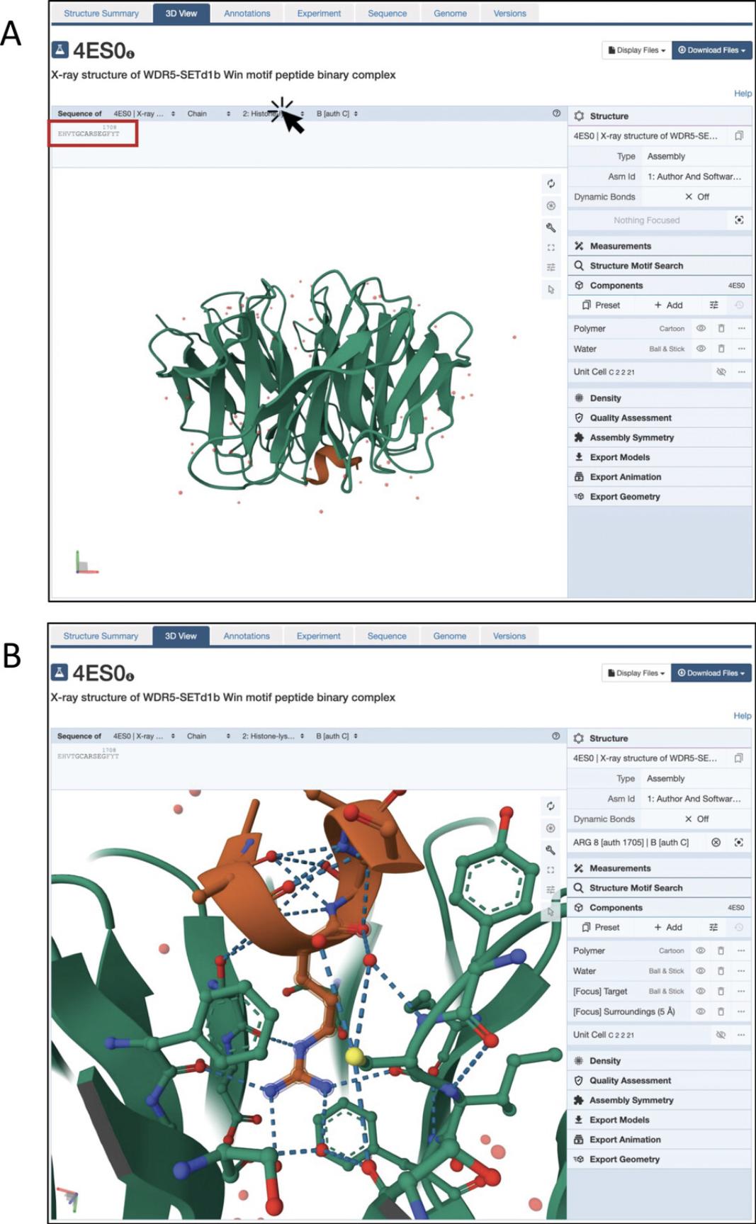
7.Identify the chain for your protein of interest. In the menu on top of the structure viewer, you can select the sequence of this chain to be displayed. For this example, click on “2: Histone-lysine N-methyltransferase SETD1B” to see its amino acid sequence (Fig. 9A). In our case, this is a very short sequence because only a small fragment of SETD1B is included in the structure. Then identify your residue of interest.
8.Once you have identified your residue, click on it to zoom in and see it in a ball-and-stick representation along with any nearby residues that may be in contact.
Analysis
9.Assess the function of the wild-type residue in its 3D context, and the effect of the substitution.
Alternate Protocol 2: USING INFORMATION FROM HOMOLOGY MODELING WITH SWISS-MODEL
Homology modeling, a precursor to AI-based modeling, infers the structure of a target protein by projecting its sequence onto the known 3D structure of a similar protein (the “template”). Although the accuracy of AlphaFold and other AI-based programs surpasses that of homology modeling, we found the SWISS-MODEL homology modeling server (Waterhouse et al., 2018) to be useful for identifying ligands, cofactors, protein-protein interactions, and potentially different conformational states of a protein.
In this protocol, we will use the AGTPBP1 Arg918Trp variant as an example to illustrate how SWISS-MODEL can be used to provide structural information on substrates, ligands, and protein multimers.
Necessary Resources
Hardware
- Computer with internet access
Software
- Standard internet browser
Files
- Amino acid sequence of your protein in FASTA format
Preparation
1.Follow steps 1-4 of the Basic Protocol to identify the consensus sequence to use (Q9UPW5-1) and gather functional information about AGTPBP1 and Arg918.
Mapping
2.Go to SWISS-MODEL (https://swissmodel.expasy.org) and click on the “Start Modelling” button on the left side of the screen.
3.Obtain the amino acid sequence of your protein and paste it in the corresponding field.
4.Click on “Search For Templates” to search for possible template structures.
<img src="https://static.yanyin.tech/literature_test/cpz1857-fig-0010-m.jpg" alt="List of potential templates found by SWISS-MODEL. Examine their properties, such as the oligomeric status in the "Oligo State" column and the bound ligands in the "Ligands” column. Select the template(s) for modeling (checkboxes on the left) and click “Build Models.” More details are available by clicking on the red template name (here: 4b6z.1.A; highlighted by the right dashed rectangle with arrowhead)." loading="lazy" title="Details are in the caption following the image"/>
5.Explore the templates’ characteristics and quality in the “Template Results” page.
6.To explore the oligomeric state of the templates, sort them by “Identity” and inspect the “Oligo State” column (excluding the AlphaFold model, which is always a monomer).
7.To explore small molecule ligands, inspect the “Ligand” column (excluding the AlphaFold model).
8.Click on the “Build Models” field above the structure viewer to make one model for each selected template.
9.After the model(s) is (are) completed, go to the results section by clicking on the “Models” tab at the top. The QMEANDisCo Local score plot and colored cartoon representation will be shown for your models (Fig. 11A).
<img src="https://static.yanyin.tech/literature_test/cpz1857-fig-0011-m.jpg" alt="Homology model for AGTPBP1, based on PDB template 4B6Z. (A) The “Model Results” page shows the quality scores for the model on the left. The "QMEANDisCO Local" plot and the colored cartoon on the right show a good confidence in the area surrounding the binding site, marked by a yellow triangle in the structure and red rectangle in the sequence (QMEANDisCO > 0.6). Clicking on the question marks brings up detailed information about each quality score. Click on the downward arrow next to “Model-Template Alignment” to display the alignment of your sequence to the selected template and per-residue quality scores (B). Clicking on Arg918 in the sequence shows this residue as a ball and sticks model in the structure viewer. The zinc ion appears as a gray sphere." loading="lazy" title="Details are in the caption following the image"/>
10.Click on the downward arrow next to “Model-Template Alignment” to see the alignment of model sequence versus template sequence, with the respective quality scores. If the residue numbers are not showing, you may resize this panel to have a better view of the sequence.
11.Select your residue of interest in the model sequence to see a closer look of the positioning and structure of this residue in its 3D context (Fig. 11B).
Analysis
12.Assess the function of the wild-type residue in its 3D context, and the effect of the substitution.
13.For better visualization, you may download the model to your computer by clicking on the “Model 01” button in the “Models” section and selecting “PDB Format.” This file can be then opened in more versatile structure viewers such as PDB Mol* viewer (see Alternate Protocol 1, step 5) or PyMOL (see Alternate Protocol 4).
Alternate Protocol 3: PREDICTING 3D STRUCTURES WITH ColabFold
Atypical isoforms, truncations, or protein-protein complexes may not be precalculated by AlphaFold or accessible through the PDB or SWISS-MODEL. In these situations, ColabFold can be used to produce structures of single and multiple protein chains. ColabFold is a free platform that provides accelerated prediction of protein structures and complexes using AlphaFold (Mirdita et al., 2022). It is hosted by Google Colaboratory, making protein folding accessible to researchers who lack the resources to install and use AlphaFold locally.
As an example, we will use ColabFold to analyze the Cys206Tyr and Val155Met variants of the STING1 protein in monomeric and dimeric conformations, respectively.
Necessary Resources
Hardware
- Computer with internet access
Software
- Standard internet browser
Preparation
1.Go to the UniProt page for human STING1 (UniProt ID Q86WV6; https://www.uniprot.org/uniprotkb/Q86WV6/entry). Scroll down to the “Sequence” section.
2.Gather functional information on the gene from UniProt.
Mapping
Accessing ColabFold
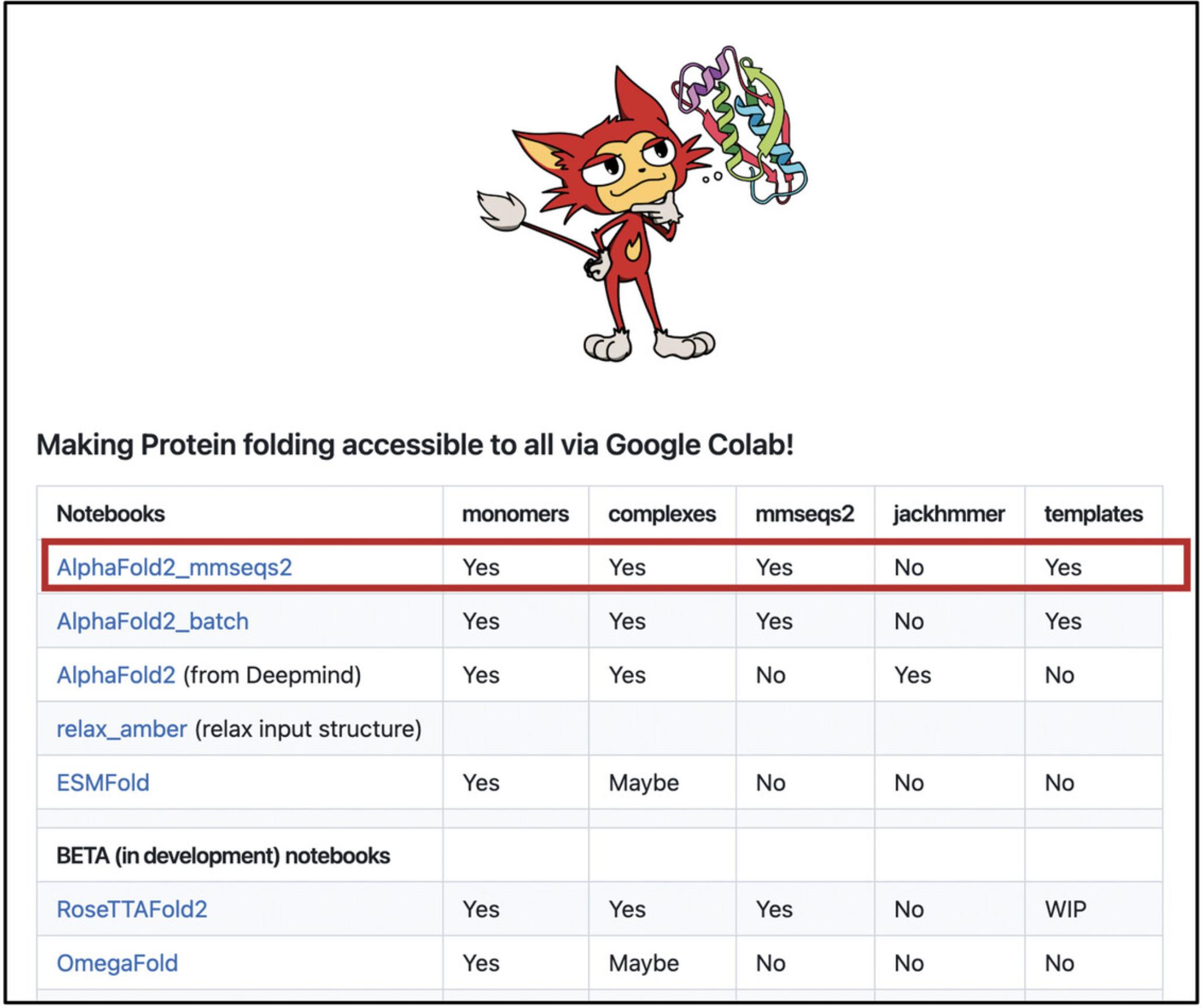
3.We recommend accessing ColabFold through its GitHub page (https://github.com/sokrypton/ColabFold) to stay updated on notebook changes and resource additions or modifications (Fig. 12). Once on that page, scroll down to the notebooks section and click on the first ColabFold notebook (currently: AlphaFold2_mmseqs2). This will open a Google Colaboratory page in your browser where you can run the code and make predictions.
Performing predictions in single protein chains
4.Obtain the sequence for the isoform of interest from the UniProt entry page.
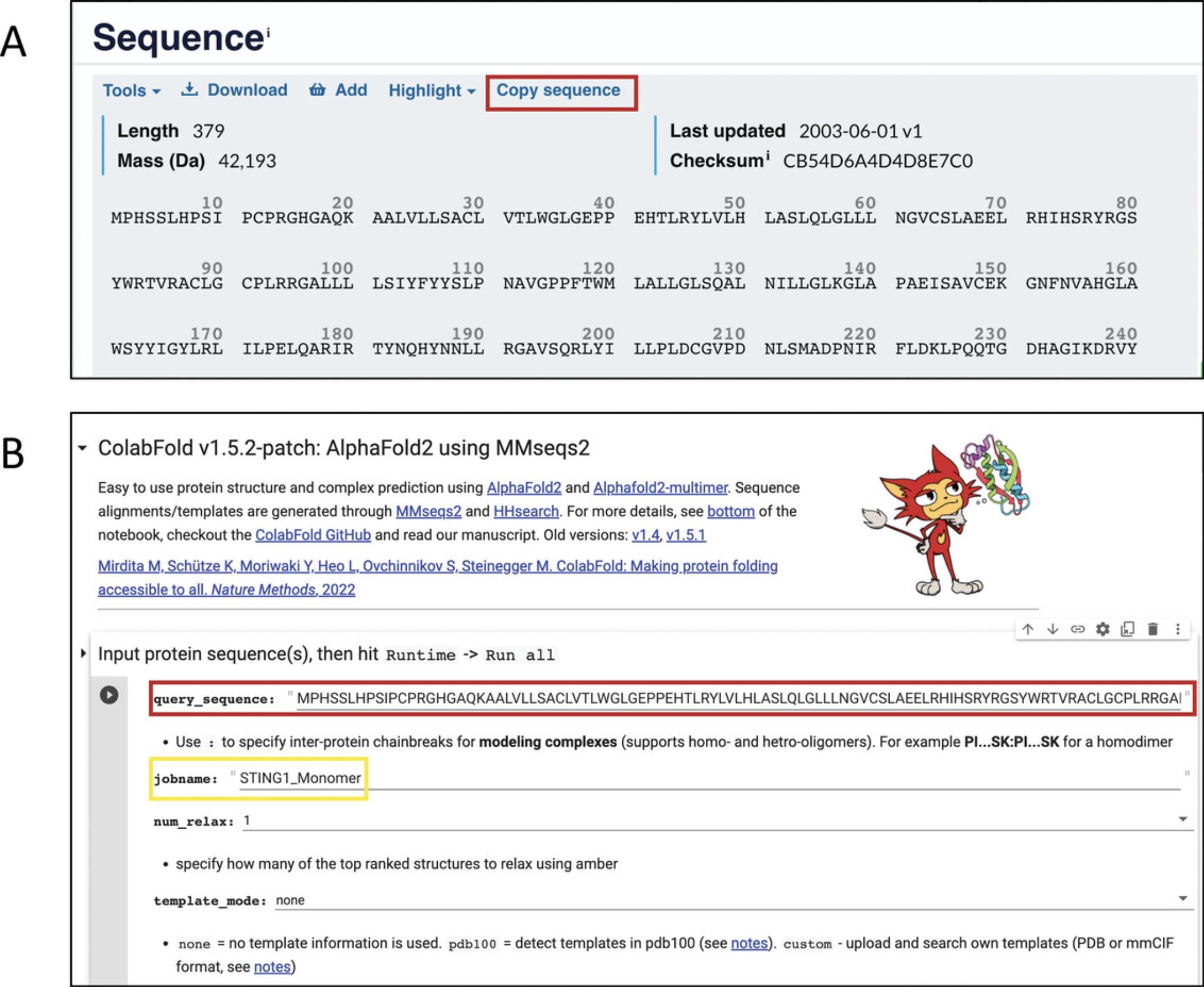
5.To run ColabFold in default mode, go to the AlphaFold2_mmseqs2 notebook (step 3), and paste the protein sequence into the “query_sequence” field of the first section titled “Input protein sequence(s)…”. Assign a name to your job in the “jobname” field (Fig. 13B, yellow rectangle).
6.In the “Input protein sequence(s)” section, set the “num_relax” parameter to either 1 (only the best-scored model will be relaxed) or 5 (all models will be relaxed). This last option takes considerably longer, but if you want to look at the conformations of amino acids in atomic detail, you should always look at a relaxed model. Changing the “template_mode” from “none” to “pdb100” in the same section may improve performance when sequences lack sufficient known homologues but have a close structure deposited in the PDB.
7.To run ColabFold, go to the Menu on the top of the notebook (below the notebook name, AlphaFold2.ipynb), click on “Runtime,” and then click on “Run all.”
8.Once your job is finished (which can take anywhere from a few minutes to a few hours), scroll down to the “Run prediction” section to evaluate the results (Fig. 14A).
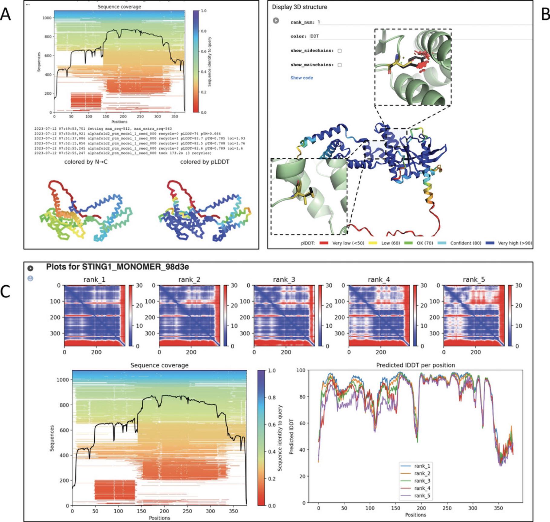
9.Assess the produced models with the interactive 3D protein viewer in the “Display 3D structure” section (Fig. 14B).
10.Evaluate the quality scores in the “Plots” section. This section displays the PAE plots, sequence coverage, and pLDDT.
Analysis
11.Once the run is finished, a compressed folder containing all of ColabFold's generated files will be automatically downloaded to your computer. You can then analyze the Cys206Tyr and Val155Met variants using the downloaded PDB files with structure viewers such as Mol* (Alternate Protocol 1, step 6) or PyMOL (Alternate Protocol 4).
Performing predictions for multimers
ColabFold also allows the analysis of homomultimers (multiple copies of the same protein chain) and heteromultimers (complex of different proteins). The process is similar to single-chain predictions, with slight differences in interpreting the results. As an example, we will model a homodimer of STING1 to analyze the gain-of-function Val155Met variant (Jeremiah et al., 2014). To do so, we perform the steps above with variations in some steps as described below.
Preparation
12.Follow steps 1 and 2 of this protocol to obtain the sequence and functional information for STING1.Open the AlphaFold2_mmseqs2 notebook as described in step 3.
Mapping
13.To model a homodimer (a protein complex consisting of two identical chains), paste the monomer sequence once into the “query-sequence” field. Then add a colon character “:” and paste the same sequence once again after the colon (Fig. 15A). Run as described in steps 6-10.
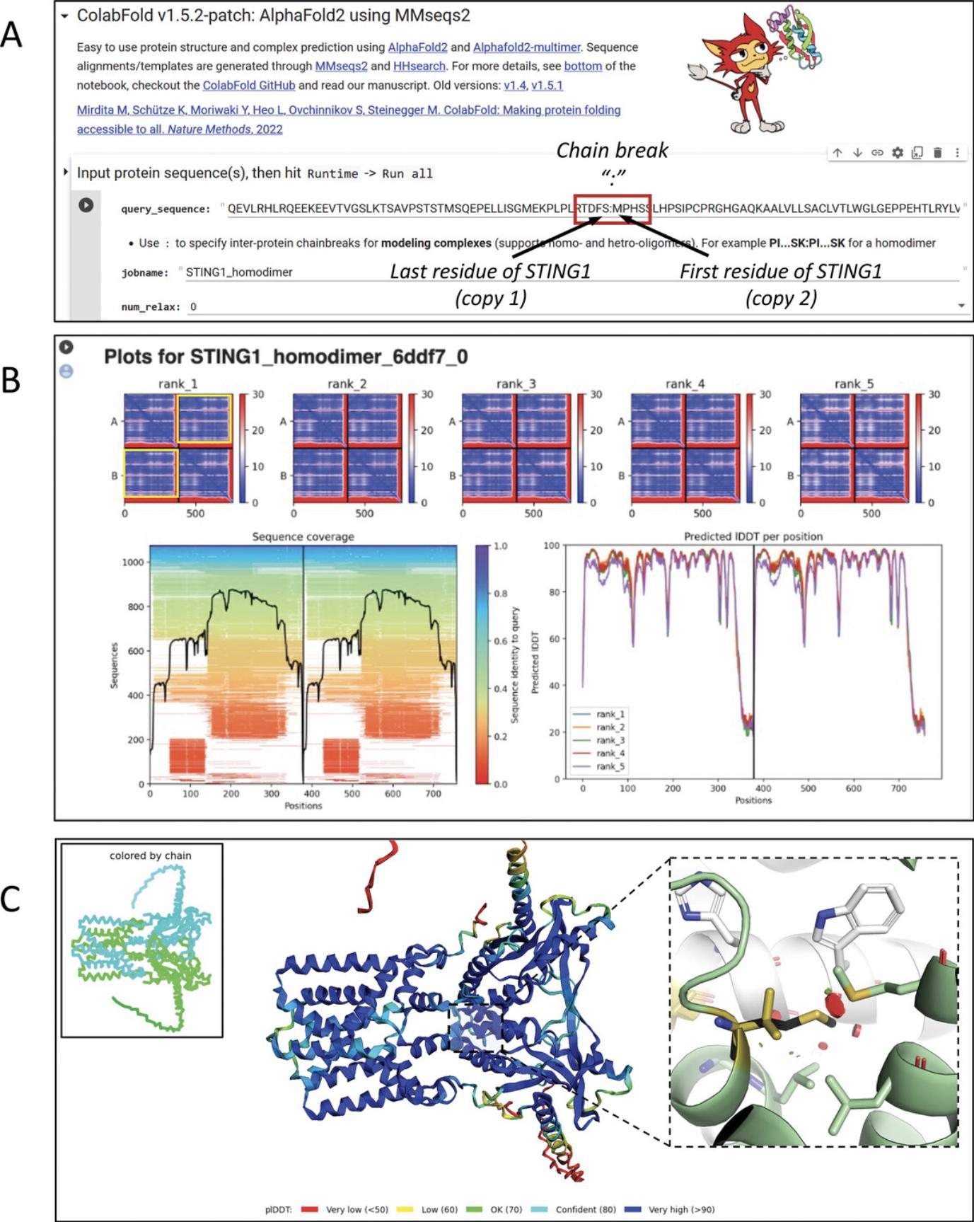
14.Assess the quality of the modeled chains and their predicted interactions.
Analysis
15.As for the monomer, once the run is finished, all of ColabFold's files will be automatically downloaded to your computer in a compressed folder. The variants can be then analyzed from the PDB files with structure viewers such as Mol* (Alternate Protocol 1, step 6) or PyMOL (Alternate Protocol 4).
Alternate Protocol 4: STRUCTURE VISUALIZATION AND ANALYSIS WITH PyMOL
The web-based structure viewers integrated in the AlphaFold or the PDB databases are sufficient for many types of structural analysis. However, specialized stand-alone visualization programs present additional tools for variant analysis and preparation of illustrative figures for presentations or manuscripts. This alternate protocol summarizes useful functions for variant analysis with PyMOL. For more features and alternative approaches, see the PyMOL support and Wiki pages at https://pymol.org/2/support.html. As an example for this protocol, we will once again look at the Arg918Trp variant in the AGTPBP1 gene.
Necessary Resources
Hardware
- Computer with internet access, 3-click mouse
Software
- PyMOL molecular visualization software. See step 3 below for installation instructions
Files
- PDB file(s) with the atomic coordinates of your protein(s) of interest
Preparation
1.Follow steps 1-4 in the Basic Protocol to identify the consensus sequence to use (Q9UPW5-1) and gather functional information about AGTPBP1 and Arg918.
Mapping
2.Download the AGTPBP1 model from the AlphaFold database (https://alphafold.ebi.ac.uk/entry/Q4U2V3).
Install PyMOL
3.There are three ways to install PyMOL on your operating system:
-
Purchase and download the pre-compiled program (or installer for Windows) fromhttps://pymol.org/2/#download.
-
Download the “Educational-use-only” PyMOL fromhttps://pymol.org/edu/. This version is freely available to teachers and high school and college students. It is easy to install, but lacks certain features, including those required to create high-quality figures for publications.
-
Install full PyMOL for free under an open-source license (https://pymolwiki.org/index.php?search=install&title=Special%3ASearch&go=Go). This requires the use of the command line.
Load and display your PDB structure
4.Launch the PyMOL application and load your PDB file.
5.To change the representation style of the object, click on the “S” menu of the object, to the far right, and choose from options such as lines, sticks, ribbon, cartoon, dots, spheres, mesh, surface, and more.
6.For publication-quality figures, we recommend using a white background. To do so, go to the top menu bar and select “Display” > “Background” > “White.”
7.To change the color of your object, click on the “C” menu and choose from the available colors. We recommend color-coding the protein by element. Select “C” > “by element” and choose the first option (“HNOS”).
8.To color AlphaFold models by their pLDDT score as in the AlphaFold database, type the following commands in the command prompt:
run https://raw.githubusercontent.com/cbalbin-bio/pymol-color-alphafold/master/coloraf.py
coloraf <model_name>
9.If the loaded PDB contain include hydrogen atoms (which is not the case for precalculated AlphaFold structures), we recommend removing them for clarity by going to “A” > “hydrogens” > “remove.”
10.To manually orient your structure, it is best to use a three-button mouse.
11.Save your session as a PyMOL session (.pse) file by clicking on “File” > “Save Session.”
Visualize the residue of interest
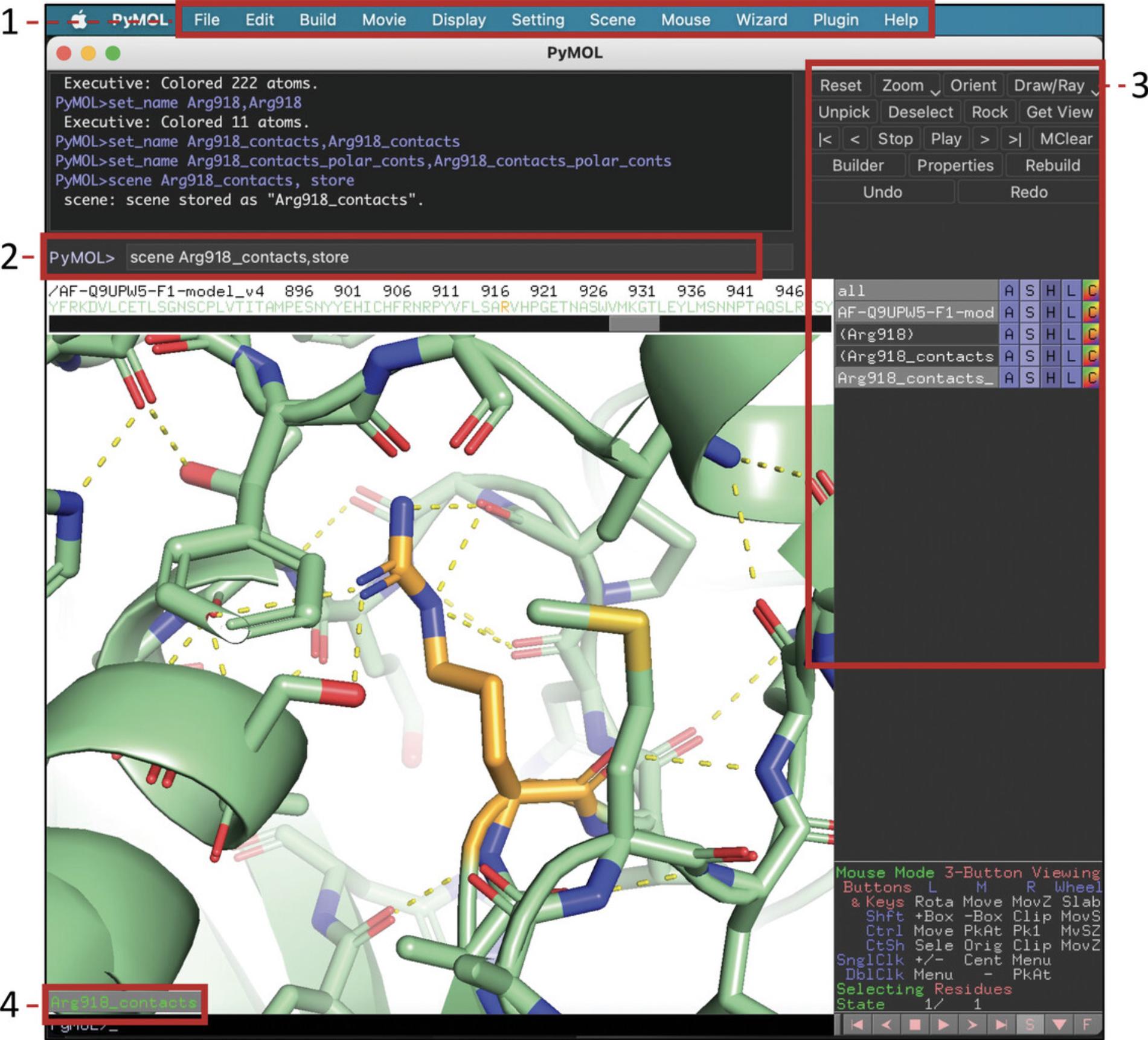
12.Display the one-letter-code sequence of the residues in the PDB file by clicking on the salmon-colored “S” in the menu on the bottom right of the window (Fig. 17, 1).
<img src="https://static.yanyin.tech/literature_test/cpz1857-fig-0017-m.jpg" alt="Mutagenesis of Arg918 (orange carbons) into Trp (black carbons) in PyMOL. Steric clashes are represented by disks. 1, Functional buttons that allow exploration of different rotamers using arrows and displaying the sequence using "S"; 2, mutagenesis tool menu." loading="lazy" title="Details are in the caption following the image"/>
13.Click on the residue of interest in the sequence field (use the gray horizontal scroll bar just below it if needed). After making this selection, a “(sele)” tab will appear in the Object Control Panel.
14.To center and/or zoom on the residue, use the commands “A” > “center ” or “zoom” next to the “Arg918” selection object. Show this residue as stick model by selecting (Arg918) “S” > sticks.
15.For our example, we colored the “AF-Q9UPW5-F1-model_v4” object in pale green (“C” > “greens” > “palegreen”), and “Arg918” in orange (“C” > “orange” > “brightorange”). Color-code the protein by element by selecting “C” > “by element” > “HNOS” next to the “AF-Q9UPW5-F1-model_v4” object (Fig. 16).
Show interactions
16.To identify residues close to Arg918, click on Arg918 (either in the structure window or the sequence pane). Then rename the new object “(sele)” into “Arg918_contacts” as described above.
17.For the object “Arg918_contacts,” click on “A” > “modify” > “expand” > “by 6 A, residues” (the range within which we want to identify interacting residues).
18.Show these contacts as sticks (“Arg918_contacts” > “S” > “sticks”).
19.To show the H-bonds between the contact residues, go to the “Arg918_contacts” selection, and click on “A” > “find” > “polar contacts” > “within selection.” A new object “Arg918_contacts_polar_conts” will appear showing the H-bonds as yellow dashed lines.
20.To see the distance in angstroms for the identified contacts, go to “Arg918_contacts_polar_conts” > “S” > “labels.” To hide them, use “H” > “labels.”
21.You can save the scene as “Arg918_contacts” (in the command line: “scene Arg918_contacts, store”).
Mutate a residue
22.To perform in silico mutagenesis on a protein, first make sure that you have no active selection by clicking into the empty space next to the structure. Then, go to “Wizard” > “Mutagenesis” > “Protein” in the top menu bar. In the Mutagenesis menu (Fig. 17, 2), click on “No Mutation” and select the amino acid that you want to mutate to (“TRP” in this example).
23.Click on Arg918 to mutate it into tryptophan. This will create a “mutation” object in the right-side object list.
24.The mutated side chain can be shown in different rotamers (i.e., preferential conformations) by using the arrows of your keyboard or the left arrow ("<") and right arrow (">") buttons at the bottom right of the screen.
25.The “mutation” object can be colored by going to “mutation” > “C.”
26.Clicking on “Apply” in the “Mutagenesis” menu (right side, lower half of the screen) will substitute the wild-type residue with the mutated residue as shown. However, to illustrate the effect of a variant, we recommend making a figure showing both residues by rendering the view without clicking “Apply” (Fig. 17; see steps 30 and 31, below).
Handle multiple chains
27.In the sequence pane, if the model has multiple chains, they are displayed one after the other in a horizontal chain sequence. Each chain is identified by a Chain ID, such as “A,” “B,” “C,” “D,” etc., in the format /<Chain_ID>/<Number…> followed by its residue positions. This is not the case for our AGTPBP1 model.
Load multiple models
28.PyMOL allows you to load and analyze multiple protein models in the same display. To load additional models, use the load command followed by the path to the model file, or drag and drop the PDB file into PyMOL (see step 4).
29.Once you have loaded multiple models, you can align them by clicking on the model you want to align and going to “A” > “align” > “to molecule (*/CA)” and selecting the target model.
Save images of your render
30.To emphasize what is in the foreground of your model, you can adjust the “fog.” To do this, hold down the shift key and right mouse button and drag the mouse to the sides to adjust the rear clipping plane. Drag the mouse toward or away from you to adjust the front clipping plane.
31.Once satisfied with the figure, click on the “Draw/Ray” button at the top right of the window and then choose your preferred figure dimensions. To adjust the ratio between them, uncheck the “Lock aspect ratio” box. Check “Transparent background” if desired. For publication-quality images, click on “Ray (slow)” to start rendering. Once complete, you are prompted to “Save Image to File” (as a .png file) or to “Copy Image to Clipboard.”
Analysis
32.Assess the function of the wild-type residue in its 3D context, and the effect of the substitution.
GUIDELINES FOR UNDERSTANDING RESULTS
The above protocols enable the user to determine the position and role of the wild-type residue within the protein's 3D structure. This makes it possible to generate hypotheses to explain how the protein's structure or function is affected by residue substitution. Below we provide a brief overview of how to understand the results in the context of protein function by discussing some of the most common cases, which are visualized in Figure 18.
1.Mutations that result in protein truncation
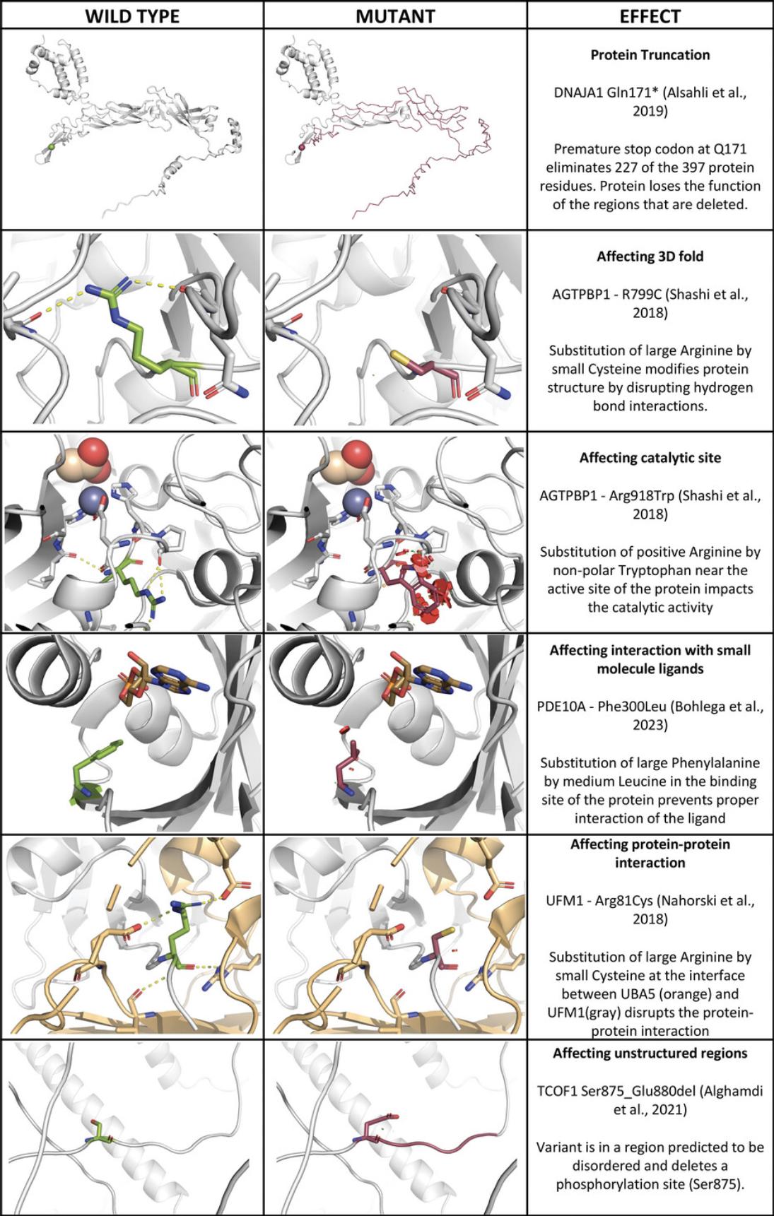
Mutations that introduce premature stop codons or frameshifts result in a truncated protein that has lost the function of the deleted regions. Structured domains that are partially deleted are likely to lose their function due to misfolding, whereas unstructured linker regions may lose their function if their remaining length is too short for their biological role (e.g., as a spacer or tether). The truncated protein domains may also be unstable due to exposed hydrophobic regions, leading to a higher degradation rate and loss of function of the remaining fragment. For example, the p.Gln171* variant in DNAJA1 eliminates 227 of the 397 protein residues, resulting in the loss of two zinc-binding motifs, most of the peptide-binding fragment, and the putative C-terminal dimerization domain (Alsahli et al., 2019). Only the J-domain and G/F-rich regions are preserved, so only functions associated with these regions would be preserved in the Gln171* variant. In rare cases, frameshift mutations can also produce novel aberrant functions (Mensah et al., 2023).
2.Mutations destabilizing the 3D protein structure
The 3D fold of a protein can be destabilized by mutations that disrupt interactions within the structure. These include:
- Hydrophobic interactions : Most 3D structures are strongly stabilized by hydrophobic interactions. A variant that replaces a hydrophobic amino acid with a polar or charged one can disrupt the hydrophobic core of a protein, destabilizing the structure or affecting protein-protein interactions.
- Electrostatic interactions : Electrostatic interactions often tether proteins at or close to the surface. A charge-changing mutation replaces a positively charged amino acid with a negatively charged amino acid, or a charged residue with an uncharged. When they disrupt stabilizing ionic bonds, these variants can destabilize protein structures or interactions. Charge-based interactions can often be partially replaced by hydrogen bonds.
- Hydrogen bonding : Protein structures are largely stabilized by an intricate network of hydrogen bonds involving side chains and the protein backbone. A variant that disrupts the hydrogen bonding networks can weaken protein folds and interactions.
- Disulfide bonds : Disulfide bonds form between two cysteine residues and contribute to protein stability. In particular, extracellular and secreted proteins depend on disulfide bonds for their stability.
- Changes in amino acid size : A variant that introduces a bulky amino acid in a folded region can cause steric clashes, hindering proper folding and stability or abolishing protein-protein interactions. Replacing a residue with a significantly smaller one can also destabilize hydrophobic cores or interactions by leaving a gap or cavity.
- Transmembrane regions : Transmembrane regions in proteins need to have a hydrophobic surface to interact with the surrounding fatty acid chains. Replacing these with polar or charged amino acids may abrogate correct membrane insertion. Transmembrane channels and transporter proteins also rely on stereochemically precise channels and protein dynamics.
3.Mutations affecting catalytic sites
Catalytic residues accelerate chemical reactions, for example by acting as acid/base catalysts, nucleophiles, or metal-ion ligands. The surrounding residues are important for substrate binding and selectivity as well as protein dynamics required for catalysis. For example, the Arg918Trp substitution in AGTPBP1 affects a loop containing residues coordinating the zinc ion in the active site. The bulkier tryptophan causes steric clashes, disrupting the shape of the active site and abrogating zinc-ion coordination (Shashi et al., 2018; Fig. 17).
4.Mutations affecting interactions with small-molecule ligands or cofactors
Small molecules typically bind to pockets in a protein's 3D structure. Variants that modify the shape, size, or electrostatic properties of such a site may weaken or abolish this interaction. For example, the Phe300Leu variant in PDE10A substitutes a large hydrophobic amino acid in the binding site with a smaller one, preventing the interaction with cAMP (Bohlega et al., 2023).
5.Mutations affecting protein-protein interactions
Proteins can interact in several ways, including stable or defined associations such as domain-domain, domain-linear peptide, and coiled-coil interactions, as well as fuzzy interactions where partners associate without forming stable complexes, as in membrane-less condensates (Alberts, 2015; Momin et al., 2022). Strong interactions resemble those that stabilize protein 3D structures and are affected by mutations in the same way. For example, the variant Arg81Cys in UFM1 is located in a tail region that binds to UBA5.The substitution of a positively charged arginine with a shorter and hydrophobic cysteine eliminates the interaction with negatively charged residues in UBA5, weakening the interaction between UFM1 and UBA5 (Nahorski et al., 2018).
6.Mutations in extended unstructured regions
In addition to participating in protein-protein interactions (see above), long, unstructured regions can serve as linkers between structured domains and play a role in protein dynamics (Borgia et al., 2018). Intrinsically flexible regions tend to be more robust against single amino acid changes than folded protein domains; however, their characteristics and functions are often altered by PTMs. Variants within these regions can disrupt or introduce binding or PTM sites, thereby affecting the regulation, activity, stability, or associations of a protein. For example, the variant Ser875_Glu880del in TCOF1 (Alghamdi et al., 2021) is located in a region predicted to be disordered. The mutation affects the disordered fourth Treacle domain by deleting four positive charges and two serines, one of which is a phosphorylation site (Ser875).
7.Additional effects
There are many more ways in which a mutation can affect a protein structure or function. For example, aggregation-enhancing variants may also inactivate associated proteins by increasing their degradation or by sequestering them in nonfunctional aggregates (Anderson et al., 2021). Mutations may also induce changes in exon usage (Chen et al., 2019). Even synonymous mutations can have negative effects on protein function by altering codon usage, which influences the speed of translation and can potentially lead to misfolding (Liu et al., 2021).
COMMENTARY
Background Information
In this protocol, we describe how to use models from the AlphaFold Protein Structure Database, PDB, SWISS-MODEL, and ColabFold. Although AlphaFold remains the gold standard for ab initio protein structure prediction, there are other AI-based algorithms available for testing. OpenFold (Ahdritz et al., 2022) and RoseTTAFold (Baek et al., 2021) have similar architecture and performance to AlphaFold and rely on deep MSAs. ESMFold (Z. Lin et al., 2023) and OmegaFold (Wu et al., 2022) are large language model (LLM)–based algorithms that do not use MSAs. Consequently, they have a faster execution than AlphaFold (ESMFold has precalculated structures for 600 million sequences!) and may perform better for proteins without homologues. However, when sufficient MSAs exist, LLM-based algorithms are currently less precise than AlphaFold. OpenFold (https://github.com/aqlaboratory/openfold), ESMFold, RoseTTAFold, and OmegaFold (https://github.com/sokrypton/ColabFold) have Colab implementations as AlphaFold does.
Currently, no AI-based algorithm can directly predict the effect of variants on a protein's structure and function. However, LLM algorithms, which do not rely on MSAs, are better positioned to achieve this in the future. One way to predict destabilizing effects is to calculate structures for a protein and its variant and compare their stability using FoldX (Schymkowitz et al., 2005). This requires a local installation of the program. In any case, a targeted experimental verification of computational predictions is the best control. It is also important to consider the biological and clinical context, such as whether the protein is part of a multiprotein complex and whether the clinical phenotype and proposed molecular mechanism agree.
Critical Parameters
Conclusions about the molecular mechanism must be evaluated based on the confidence in the 3D model employed. For AlphaFold models, critical parameters include the MSA depth (the number of homologous sequences found), AlphaFold's predicted local distance difference test (pLDDT; should be >90 for atomistic conclusions), and the predicted aligned error (PAE; should be <5 Å for interacting protein regions).
Advanced parameters
Table 3 lists some of the parameters that more advanced users may want to tweak to try to obtain better-quality models from ColabFold.
Suggestions for further analysis
As an alternative, or support, several integrated structure-based variant analysis servers are available: for example, MISCAST (missense variant to protein structure analysis web suite, http://miscast.broadinstitute.org/; Iqbal et al., 2020), G2S (https://g2s.genomenexus.org/; Wang et al., 2018), and VarQ (https://varq.qb.fcen.uba.ar/; Radusky et al., 2018).
In addition to structural analysis, there are many other freely accessible web-based bioinformatic servers that can support variant analysis. In addition to those mentioned in the Introduction, and Phobius (see Basic Protocol.2), there is the Eukaryotic Linear Motif (ELM) resource (http://elm.eu.org/index.html; Kumar et al., 2020) for identifying functional sequences, Fuzdrop (https://fuzdrop.bio.unipd.it/predictorl; Hardenberg et al., 2020) for identifying regions likely to phase separate, and DISOPRED (http://bioinf.cs.ucl.ac.uk/psipredl; Jones & Cozzetto, 2015) to aid in the prediction of disordered regions in a protein sequence. ConSurf (http://consurf.tau.ac.il/; Ashkenazy et al., 2016) calculates conservation scores for every residue along a sequence and provides useful visualizations.
Troubleshooting
For a full list of troubleshooting suggestions, known issues, and limitations of the ColabFold program, please refer to the corresponding sections in the AlphaFold2_mmseqs2 notebook or the FAQ section in the GitHub repository (https://github.com/sokrypton/ColabFold). Table 2 shows two of the most common issues encountered by users.
| Problem | Possible cause | Solution |
|---|---|---|
| Your session crashed after using all available RAM | The model that you are trying to build is too large, and you don't have enough RAM allocated. | Split your protein into domains (see the “Family & Domains” section in step 4 of the Basic Protocol) and run each domain separately. The maximum sequence length that you can run in ColabFold varies from session to session and ranges from 1000 to 2000 residues (all protein chains combined). |
| Runtime disconnected: Your runtime has been disconnected due to inactivity or reaching its maximum duration | (a) The program has been running for more than 12 hr or (b) the page has been sitting idle for too long after finishing the run or stopping due to an error. | If the program exceeded its run time limit of 12 hr, you should split the sequence into domains and run those separately. Otherwise, just click on the Reconnect button. |
| Parameter | Possible values | Description | How/when to use it |
|---|---|---|---|
| Msa_mode | mmseqs2_uniref_env (default) mmseqs2_uniref single_sequence custom |
The MSA database that will be used to search against. |
mmseqs2_uniref_env: Search against the UniRef and environmental datasets mmseqs2_uniref: Search only against very well curated/annotated data from UniRef. Warning: May not find enough sequences. single_sequence: Disables MSA information. Recommended for de-novo-designed sequences or cases where not many homologs are expected. custom: Use if you have constructed your own MSA |
| Num_recycles | Integer from 0 to 48 | Number of times to recycle the outputs through the network before assembling the final models. Sometimes higher recycles can give better results. | If the model that you obtained with the default parameters is not satisfactory, you can try increasing the number of recycles to get a better result. |
| recycle_early_stop_tolerance | auto, 0.0, 0.5, and 1.0 | If the difference in angstroms from the coordinates obtained in two consecutive recycles is lower than this number, the program will stop and the final model will be produced. | If you set a high number of recycles you can use this parameter to stop the program if there is not a noticeable progress from one recycle to the next. |
| max_msa | Pair of integers to select from dropdown list: 512:1024, 256:512, 64:128, 32:64, 16:32 | Different options to restrict the size of the MSA | If you want to attempt to get more diversity in the models created (at the potential cost of less confidence), reduce the values of this parameter. |
| Num_seed | Integer from 1 to 16 | Increase the number of random seeds to generate models. | If you want to attempt to get more diversity in the models created, increase this value. |
Acknowledgments
This research was supported by the King Abdullah University of Science and Technology (KAUST) through the baseline fund and Award No. FCC/1/1976-33, URF/1/4379-01 and REI/1/4446-01 from the Office of Sponsored Research (OSR). For computer time, this research used the resources of the Supercomputing Laboratory at King Abdullah University of Science & Technology (KAUST) in Thuwal, Saudi Arabia.
Author Contributions
Francisco J. Guzmán-Vega : Conceptualization, methodology, project administration, supervision, writing—original draft, writing—review and editing. Ana C. González-Álvarez : Investigation, software, visualization, writing—original draft. Karla A. Peña-Guerra : Investigation, software, visualization, writing—original draft. Kelly J. Cardona-Londoño : Investigation, software, visualization, writing—original draft. Stefan T. Arold : Conceptualization, project administration, supervision, validation, writing—review and editing.
Conflict of Interest
The authors declare no conflict of interest.
Open Research
Data Availability Statement
Data sharing is not applicable to this article as no new data were created or analyzed in this study.
Literature Cited
- Adzhubei, I., Jordan, D. M., & Sunyaev, S. R. (2013). Predicting functional effect of human missense mutations using PolyPhen-2. Current Protocols in Human Genetics , 76(1), 7.20.1–7.20.41. https://doi.org/10.1002/0471142905.hg0720s76
- Adzhubei, I., Schmidt, S., Peshkin, L., Ramensky, V. E., Gerasimova, A., Bork, P., Kondrashov, A. S., & Sunyaev, S. R. (2010). A method and server for predicting damaging missense mutations. Nature Methods , 7(4), 248–249. https://doi.org/10.1038/nmeth0410-248
- Ahdritz, G., Bouatta, N., Kadyan, S., Xia, Q., Gerecke, W., O'Donnell, T. J., Berenberg, D., Fisk, I., Zanichelli, N., Zhang, B., Nowaczynski, A., Wang, B., Stepniewska-Dziubinska, M. M., Zhang, S., Ojewole, A., Guney, M. E., Biderman, S., Watkins, A. M., Ra, S., … AlQuraishi, M. (2022). OpenFold: Retraining AlphaFold2 yields new insights into its learning mechanisms and capacity for generalization. BioRxiv , 517210. https://doi.org/10.1101/2022.11.20.517210
- Alberts, B. (2015). Molecular biology of the cell ( 6th ed.). Garland Science, Taylor and Francis Group.
- Alghamdi, M. A., Mulla, J., Saheb Sharif-Askari, N., Guzmán-Vega, F. J., Arold, S. T., Abd-Alwahed, M., Alharbi, N., Kashour, T., & Halwani, R. (2021). A novel biallelic STING1 gene variant causing SAVI in two siblings. Frontiers in Immunology , 11, 599564. https://doi.org/10.3389/fimmu.2020.599564
- Alghamdi, M., Alhumsi, T. R., Altweijri, I., Alkhamis, W. H., Barasain, O., Cardona-Londoño, K. J., Ramakrishnan, R., Guzmán-Vega, F. J., Arold, S. T., Ali, G., Adly, N., Ali, H., Basudan, A., & Bakhrebah, M. A. (2021). Clinical and genetic characterization of craniosynostosis in Saudi Arabia. Frontiers in Pediatrics , 9, 582816. https://doi.org/10.3389/fped.2021.582816
- Alsahli, S., Alfares, A., Guzmán-Vega, F. J., Arold, S. T., Ba-Armah, D., & Al Mutairi, F. (2019). Truncating biallelic variant in DNAJA1, encoding the co-chaperone Hsp40, is associated with intellectual disability and seizures. Neurogenetics , 20(2), 109–115. https://doi.org/10.1007/s10048-019-00573-6
- Anderson, C. L., Langer, E. R., Routes, T. C., McWilliams, S. F., Bereslavskyy, I., Kamp, T. J., & Eckhardt, L. L. (2021). Most myopathic lamin variants aggregate: A functional genomics approach for assessing variants of uncertain significance. NPJ Genomic Medicine , 6(1), 103. https://doi.org/10.1038/s41525-021-00265-x
- Ashkenazy, H., Abadi, S., Martz, E., Chay, O., Mayrose, I., Pupko, T., & Ben-Tal, N. (2016). ConSurf 2016: An improved methodology to estimate and visualize evolutionary conservation in macromolecules. Nucleic Acids Research , 44(W1), W344–350. https://doi.org/10.1093/nar/gkw408
- Backman, J. D., Li, A. H., Marcketta, A., Sun, D., Mbatchou, J., Kessler, M. D., Benner, C., Liu, D., Locke, A. E., Balasubramanian, S., Yadav, A., Banerjee, N., Gillies, C. E., Damask, A., Liu, S., Bai, X., Hawes, A., Maxwell, E., Gurski, L., … Ferreira, M. A. R. (2021). Exome sequencing and analysis of 454,787 UK Biobank participants. Nature , 599(7886), 628–634. https://doi.org/10.1038/s41586-021-04103-z
- Baek, M., DiMaio, F., Anishchenko, I., Dauparas, J., Ovchinnikov, S., Lee, G. R., Wang, J., Cong, Q., Kinch, L. N., Schaeffer, R. D., Millán, C., Park, H., Adams, C., Glassman, C. R., DeGiovanni, A., Pereira, J. H., Rodrigues, A. V., van Dijk, A. A., Ebrecht, A. C., … Baker, D. (2021). Accurate prediction of protein structures and interactions using a three-track neural network. Science , 373(6557), 871–876. https://doi.org/10.1126/science.abj8754
- Bohlega, S., Abusrair, A. H., Al-Qahtani, Z., Guzmán-Vega, F. J., Ramakrishnan, R., Aldosari, H., Aldakheel, A., Al-Qahtani, S., Monies, D., & Arold, S. T. (2023). Expanding the genotype-phenotype landscape of PDE10A-associated movement disorders. Parkinsonism & Related Disorders, 108, 105323. https://doi.org/10.1016/j.parkreldis.2023.105323
- Borgia, A., Borgia, M. B., Bugge, K., Kissling, V. M., Heidarsson, P. O., Fernandes, C. B., Sottini, A., Soranno, A., Buholzer, K. J., Nettels, D., Kragelund, B. B., Best, R. B., & Schuler, B. (2018). Extreme disorder in an ultrahigh-affinity protein complex. Nature , 555(7694), 61–66. https://doi.org/10.1038/nature25762
- Brandes, N., Goldman, G., Wang, C. H., Ye, C. J., & Ntranos, V. (2022). Genome-wide prediction of disease variants with a deep protein language model [Preprint]. bioRxiv , 505311. https://doi.org/10.1101/2022.08.25.505311
- Chen, K., Lu, Y., Zhao, H., & Yang, Y. (2019). Predicting the change of exon splicing caused by genetic variant using support vector regression. Human Mutation , 40(9), 1235–1242. https://doi.org/10.1002/humu.23785
- Frazer, J., Notin, P., Dias, M., Gomez, A., Min, J. K., Brock, K., Gal, Y., & Marks, D. S. (2021). Disease variant prediction with deep generative models of evolutionary data. Nature , 599(7883), 91–95. https://doi.org/10.1038/s41586-021-04043-8
- Hardenberg, M., Horvath, A., Ambrus, V., Fuxreiter, M., & Vendruscolo, M. (2020). Widespread occurrence of the droplet state of proteins in the human proteome. Proceedings of the National Academy of Sciences , 117(52), 33254–33262. https://doi.org/10.1073/pnas.2007670117
- Iqbal, S., Hoksza, D., Pérez-Palma, E., May, P., Jespersen, J. B., Ahmed, S. S., Rifat, Z. T., Heyne, H. O., Rahman, M. S., Cottrell, J. R., Wagner, F. F., Daly, M. J., Campbell, A. J., & Lal, D. (2020). MISCAST: MIssense variant to protein StruCture analysis web SuiTe. Nucleic Acids Research , 48(W1), W132–W139. https://doi.org/10.1093/nar/gkaa361
- Ittisoponpisan, S., Islam, S. A., Khanna, T., Alhuzimi, E., David, A., & Sternberg, M. J. E. (2019). Can predicted protein 3D structures provide reliable insights into whether missense variants are disease associated? Journal of Molecular Biology , 431(11), 2197–2212. https://doi.org/10.1016/j.jmb.2019.04.009
- Jeremiah, N., Neven, B., Gentili, M., Callebaut, I., Maschalidi, S., Stolzenberg, M.-C., Goudin, N., Frémond, M.-L., Nitschke, P., Molina, T. J., Blanche, S., Picard, C., Rice, G. I., Crow, Y. J., Manel, N., Fischer, A., Bader-Meunier, B., & Rieux-Laucat, F. (2014). Inherited STING-activating mutation underlies a familial inflammatory syndrome with lupus-like manifestations. The Journal of Clinical Investigation , 124(12), 5516–5520. https://doi.org/10.1172/JCI79100
- Jones, D. T., & Cozzetto, D. (2015). DISOPRED3: Precise disordered region predictions with annotated protein-binding activity. Bioinformatics , 31(6), 857–863. https://doi.org/10.1093/bioinformatics/btu744
- Jumper, J., Evans, R., Pritzel, A., Green, T., Figurnov, M., Ronneberger, O., Tunyasuvunakool, K., Bates, R., Žídek, A., Potapenko, A., Bridgland, A., Meyer, C., Kohl, S. A. A., Ballard, A. J., Cowie, A., Romera-Paredes, B., Nikolov, S., Jain, R., Adler, J., … Hassabis, D. (2021). Highly accurate protein structure prediction with AlphaFold. Nature , 596(7873), 583–589. https://doi.org/10.1038/s41586-021-03819-2
- Kumar, M., Gouw, M., Michael, S., Sámano-Sánchez, H., Pancsa, R., Glavina, J., Diakogianni, A., Valverde, J. A., Bukirova, D., Čalyševa, J., Palopoli, N., Davey, N. E., Chemes, L. B., & Gibson, T. J. (2020). ELM—the eukaryotic linear motif resource in 2020. Nucleic Acids Research , 48(D1), D296–D306. https://doi.org/10.1093/nar/gkz1030
- Laskowski, R. A., Stephenson, J. D., Sillitoe, I., Orengo, C. A., & Thornton, J. M. (2020). VarSite: Disease variants and protein structure. Protein Science , 29(1), 111–119. https://doi.org/10.1002/pro.3746
- Lin, W., Wells, J., Wang, Z., Orengo, C., & Martin, A. C. R. (2023). VariPred: Enhancing pathogenicity prediction of missense variants using protein language models [Preprint]. bioRxiv , 532942. https://doi.org/10.1101/2023.03.16.532942
- Lin, Z., Akin, H., Rao, R., Hie, B., Zhu, Z., Lu, W., Smetanin, N., Verkuil, R., Kabeli, O., Shmueli, Y., dos Santos Costa, A., Fazel-Zarandi, M., Sercu, T., Candido, S., & Rives, A. (2023). Evolutionary-scale prediction of atomic-level protein structure with a language model. Science , 379(6637), 1123–1130. https://doi.org/10.1126/science.ade2574
- Liu, Y., Yang, Q., & Zhao, F. (2021). Synonymous but not silent: The codon usage code for gene expression and protein folding. Annual Review of Biochemistry , 90(1), 375–401. https://doi.org/10.1146/annurev-biochem-071320-112701
- MacArthur, D. G., Manolio, T. A., Dimmock, D. P., Rehm, H. L., Shendure, J., Abecasis, G. R., Adams, D. R., Altman, R. B., Antonarakis, S. E., Ashley, E. A., Barrett, J. C., Biesecker, L. G., Conrad, D. F., Cooper, G. M., Cox, N. J., Daly, M. J., Gerstein, M. B., Goldstein, D. B., Hirschhorn, J. N., … Gunter, C. (2014). Guidelines for investigating causality of sequence variants in human disease. Nature , 508(7497), 469–476. https://doi.org/10.1038/nature13127
- Melki, I., Rose, Y., Uggenti, C., van Eyck, L., Frémond, M.-L., Kitabayashi, N., Rice, G. I., Jenkinson, E. M., Boulai, A., Jeremiah, N., Gattorno, M., Volpi, S., Sacco, O., Terheggen-Lagro, S. W. J., Tiddens, H. A. W. M., Meyts, I., Morren, M.-A., de Haes, P., Wouters, C., … Crow, Y. J. (2017). Disease-associated mutations identify a novel region in human STING necessary for the control of type I interferon signaling. Journal of Allergy and Clinical Immunology , 140(2), 543–552.e5. https://doi.org/10.1016/j.jaci.2016.10.031
- Mensah, M. A., Niskanen, H., Magalhaes, A. P., Basu, S., Kircher, M., Sczakiel, H. L., Reiter, A. M. V., Elsner, J., Meinecke, P., Biskup, S., Chung, B. H. Y., Dombrowsky, G., Eckmann-Scholz, C., Hitz, M. P., Hoischen, A., Holterhus, P.-M., Hülsemann, W., Kahrizi, K., Kalscheuer, V. M., … Hnisz, D. (2023). Aberrant phase separation and nucleolar dysfunction in rare genetic diseases. Nature , 614(7948), 564–571. https://doi.org/10.1038/s41586-022-05682-1
- Mirdita, M., Schütze, K., Moriwaki, Y., Heo, L., Ovchinnikov, S., & Steinegger, M. (2022). ColabFold: Making protein folding accessible to all. Nature Methods , 19(6), 679–682. https://doi.org/10.1038/s41592-022-01488-1
- Momin, A. A., Mendes, T., Barthe, P., Faure, C., Hong, S., Yu, P., Kadaré, G., Jaremko, M., Girault, J.-A., Jaremko, Ł., & Arold, S. T. (2022). PYK2 senses calcium through a disordered dimerization and calmodulin-binding element. Communications Biology , 5(1), 800. https://doi.org/10.1038/s42003-022-03760-8
- Morales, J., Pujar, S., Loveland, J. E., Astashyn, A., Bennett, R., Berry, A., Cox, E., Davidson, C., Ermolaeva, O., Farrell, C. M., Fatima, R., Gil, L., Goldfarb, T., Gonzalez, J. M., Haddad, D., Hardy, M., Hunt, T., Jackson, J., Joardar, V. S., … Murphy, T. D. (2022). A joint NCBI and EMBL-EBI transcript set for clinical genomics and research. Nature , 604(7905), 310–315. https://doi.org/10.1038/s41586-022-04558-8
- Nahorski, M. S., Maddirevula, S., Ishimura, R., Alsahli, S., Brady, A. F., Begemann, A., Mizushima, T., Guzmán-Vega, F. J., Obata, M., Ichimura, Y., Alsaif, H. S., Anazi, S., Ibrahim, N., Abdulwahab, F., Hashem, M., Monies, D., Abouelhoda, M., Meyer, B. F., Alfadhel, M., … Alkuraya, F. S. (2018). Biallelic UFM1 and UFC1 mutations expand the essential role of ufmylation in brain development. Brain , 141(7), 1934–1945. https://doi.org/10.1093/brain/awy135
- Ng, P. C., & Henikoff, S. (2001). Predicting deleterious amino acid substitutions. Genome Research , 11(5), 863–874. https://doi.org/10.1101/gr.176601
- Ouyang, S., Song, X., Wang, Y., Ru, H., Shaw, N., Jiang, Y., Niu, F., Zhu, Y., Qiu, W., Parvatiyar, K., Li, Y., Zhang, R., Cheng, G., & Liu, Z.-J. (2012). Structural analysis of the STING adaptor protein reveals a hydrophobic dimer interface and mode of cyclic di-GMP binding. Immunity , 36(6), 1073–1086. https://doi.org/10.1016/j.immuni.2012.03.019
- Qi, H., Zhang, H., Zhao, Y., Chen, C., Long, J. J., Chung, W. K., Guan, Y., & Shen, Y. (2021). MVP predicts the pathogenicity of missense variants by deep learning. Nature Communications , 12(1), 510. https://doi.org/10.1038/s41467-020-20847-0
- Radusky, L., Modenutti, C., Delgado, J., Bustamante, J. P., Vishnopolska, S., Kiel, C., Serrano, L., Marti, M., & Turjanski, A. (2018). VarQ: A tool for the structural and functional analysis of human protein variants. Frontiers in Genetics , 9, 620. https://doi.org/10.3389/fgene.2018.00620
- Rentzsch, P., Witten, D., Cooper, G. M., Shendure, J., & Kircher, M. (2018). CADD: Predicting the deleteriousness of variants throughout the human genome. Nucleic Acids Research , 47(D1), D886–D894. https://doi.org/10.1093/nar/gky1016
- Schymkowitz, J., Borg, J., Stricher, F., Nys, R., Rousseau, F., & Serrano, L. (2005). The FoldX web server: An online force field. Nucleic Acids Research , 33(suppl_2), W382–W388. https://doi.org/10.1093/nar/gki387
- Shashi, V., Magiera, M. M., Klein, D., Zaki, M., Schoch, K., Rudnik-Schöneborn, S., Norman, A., Lopes Abath Neto, O., Dusl, M., Yuan, X., Bartesaghi, L., de Marco, P., Alfares, A. A., Marom, R., Arold, S. T., Guzmán-Vega, F. J., Pena, L. D., Smith, E. C., Steinlin, M., … Senderek, J. (2018). Loss of tubulin deglutamylase CCP1 causes infantile-onset neurodegeneration. The EMBO Journal , 37(23), e100540. https://doi.org/10.15252/embj.2018100540
- Tunyasuvunakool, K., Adler, J., Wu, Z., Green, T., Zielinski, M., Žídek, A., Bridgland, A., Cowie, A., Meyer, C., Laydon, A., Velankar, S., Kleywegt, G. J., Bateman, A., Evans, R., Pritzel, A., Figurnov, M., Ronneberger, O., Bates, R., Kohl, S. A. A., … Hassabis, D. (2021). Highly accurate protein structure prediction for the human proteome. Nature , 596(7873), 590–596. https://doi.org/10.1038/s41586-021-03828-1
- Varadi, M., Anyango, S., Deshpande, M., Nair, S., Natassia, C., Yordanova, G., Yuan, D., Stroe, O., Wood, G., Laydon, A., Žídek, A., Green, T., Tunyasuvunakool, K., Petersen, S., Jumper, J., Clancy, E., Green, R., Vora, A., Lutfi, M., … Velankar, S. (2021). AlphaFold protein structure database: Massively expanding the structural coverage of protein-sequence space with high-accuracy models. Nucleic Acids Research , 50(D1), D439–D444. https://doi.org/10.1093/nar/gkab1061
- Wang, J., Sheridan, R., Sumer, S. O., Schultz, N., Xu, D., & Gao, J. (2018). G2S: A web-service for annotating genomic variants on 3D protein structures. Bioinformatics , 34(11), 1949–1950. https://doi.org/10.1093/bioinformatics/bty047
- Waterhouse, A., Bertoni, M., Bienert, S., Studer, G., Tauriello, G., Gumienny, R., Heer, F. T., de Beer, T. A. P., Rempfer, C., Bordoli, L., Lepore, R., & Schwede, T. (2018). SWISS-MODEL: homology modelling of protein structures and complexes. Nucleic Acids Research , 46(W1), W296–W303 (2018). https://doi.org/10.1093/nar/gky427
- Weerts, M. J. A., Lanko, K., Guzmán-Vega, F. J., Jackson, A., Ramakrishnan, R., Cardona-Londoño, K. J., Peña-Guerra, K. A., van Bever, Y., van Paassen, B. W., Kievit, A., van Slegtenhorst, M., Allen, N. M., Kehoe, C. M., Robinson, H. K., Pang, L., Banu, S. H., Zaman, M., Efthymiou, S., Houlden, H., … Barakat, T. S. (2021). Delineating the molecular and phenotypic spectrum of the SETD1B-related syndrome. Genetics in Medicine , 23(11), 2122–2137. https://doi.org/10.1038/s41436-021-01246-2
- Wu, R., Ding, F., Wang, R., Shen, R., Zhang, X., Luo, S., Su, C., Wu, Z., Xie, Q., Berger, B., Ma, J., & Peng, J. (2022). High-resolution de novo structure prediction from primary sequence. bioRxiv , 500999. https://doi.org/10.1101/2022.07.21.500999
- Zhang, J., Vancea, A. I., & Arold, S. T. (2022). Targeting plant UBX proteins: AI-enhanced lessons from distant cousins. Trends in Plant Science , 27(11), 1099–1108. https://doi.org/10.1016/j.tplants.2022.05.012
Internet Resources
- https://www.uniprot.org/
- UniProt: protein sequence database with functional and structural information.
- https://alphafold.ebi.ac.uk/
- Database of protein structures precalculated by AlphaFold.
- https://www.rcsb.org/
- Protein Data Bank (PDB): Database containing coordinates and information on experimental macromolecular structures.
- https://swissmodel.expasy.org/
- SWISS-MODEL: Online server for homology modeling; useful for retrieving information on ligands and macromolecular complexes.
- https://github.com/sokrypton/ColabFold
- ColabFold: github page listing available Colab notebooks.
- https://www.rcsb.org/3d-view
- Mol* 3D Viewer: Web-based structure viewer.
- https://pymolwiki.org/
- PyMOL Wiki: Wikipedia page for PyMOL.

