Tracing DNA paths and RNA profiles in cultured cells and tissues with ORCA

Leslie J. Mateo, Nasa Sinnott-Armstrong, Alistair N. Boettiger

Published: 2021-02-21 DOI: 10.1038/s41596-020-00478-x

Extended

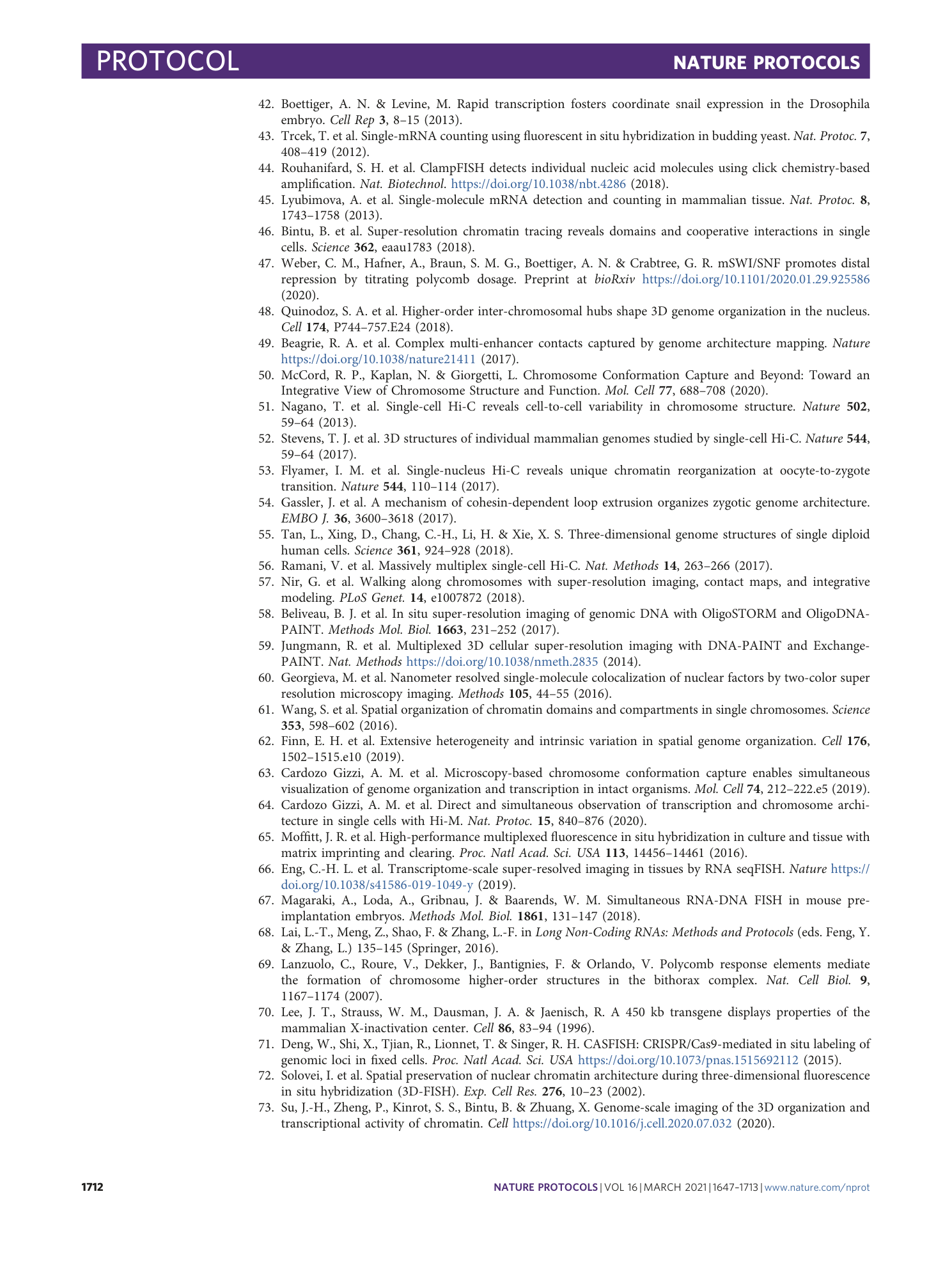
Extended Data Fig. 1 Distinct intronic RNA patterns in cryosectioned tissue.

A zoomed-in image of the most posterior body segments of a 10-12 hpf Drosophila embryo. With multiplex RNA labeling, we targeted the following RNA introns: Antp (green), abd-A (yellow), Abd-B (red), inv (blue). Note that these introns have distinct RNA patterns.

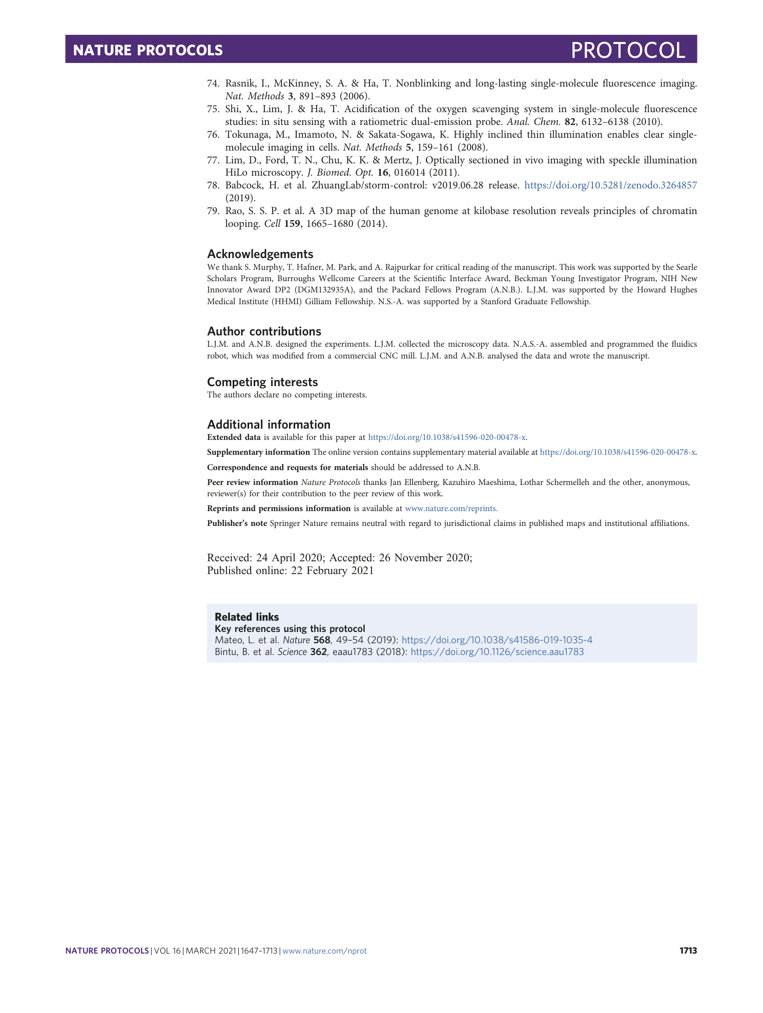
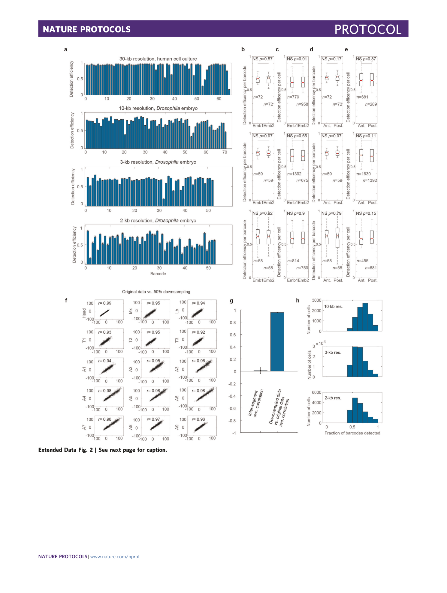
Extended Data Fig. 2 Barcode detection efficiency.

Figure modified from previous publication 25 . a , The average detection efficiency of each barcode is shown for probe sets with the resolution and cell type indicated. Error bars represent standard error of the mean. n = 1,979 cells, n = 8,801 cells, n = 94,300 cells, and n = 15,230 cells for the 30-kb, 10-kb, 3-kb, and 2-kb probesets, respectively. b , Box-and-whisker plots comparing the distribution of detection efficiencies across barcodes between two different embryos. N.S. indicates not statistically significant (two-sided Wilcoxon test, p-values indicated). For the boxplots in (b-e), the red line marks the median, the upper and lower limits of the box mark the interquartile range, and the whiskers extend to the furthest datum within 1.5 times the interquartile range. Notches denote the 95% confidence interval around the median. Sample size (n) is indicated. c , Comparison of the distribution of detection efficiencies between cells of different embryos. d , Comparison of the detection efficiency across barcodes between anterior and posterior cells. e , Comparisons of the detection efficiency across all cells between anterior and posterior cells. Results are shown for the 10-kb, 3-kb and 2-kb probesets as indicated. f , Correlation between normalized distance data from different cell types and a modified dataset in which 50% of detected barcodes were removed at random to simulate a high missed detection rate. The correlation coefficients are indicated (Pearson), computed using all unique combinations of 52 barcodes. g , Bar graph comparing the mean correlation between matched segments in the original and downsampled data shown in (f) compared to the mean inter-segment correlation. The correlation coefficients are indicated (Pearson), computed using all unique combinations of 52 barcodes. All 15 matched segment pairs shown in f are plotted compared to all 210 inter-segment pairs. This illustrates that the difference between the substantially downsampled data and the original measurements are much more similar than the typical differences between segments, demonstrating the robustness of the segment-specific findings to missing data. Error bars denote standard error of the mean. h , Histogram showing the detection efficiency per cell for each probeset.

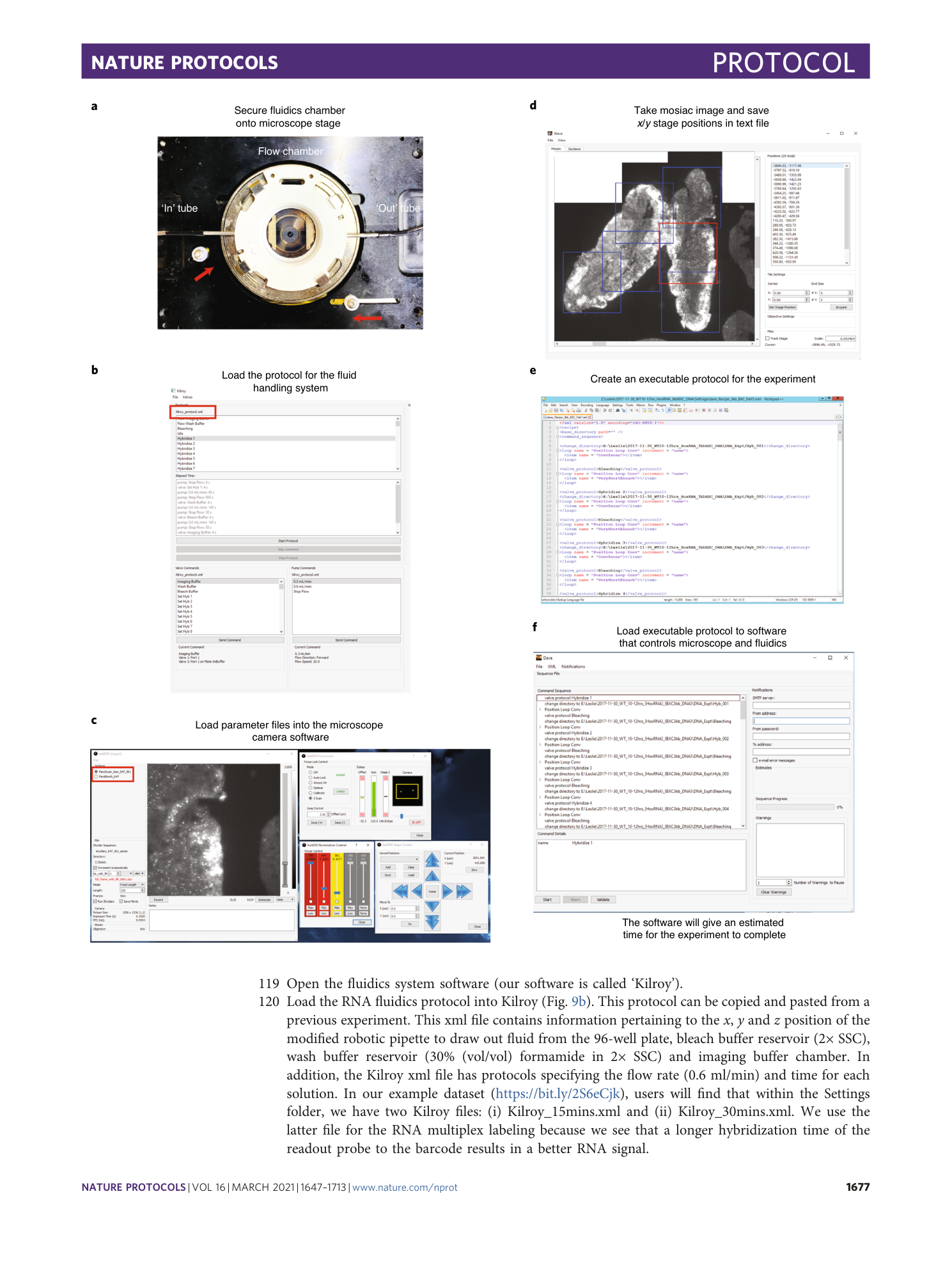
Extended Data Fig. 3 Setting up the flow chamber.

a , Layout of all the components that are needed to assemble the flow chamber. Before using, clean all components with a kimwipe that is slightly damp with ultra-pure water. Note that the 400 mm coverslip is marked with an alcohol-resistant pen. The marks indicate the location of the embryos, which are cryosectioned between the two lines in the center of the coverslip. This space is determined by the middle area of gasket 2. We also used the pen to label that our sample is WT. We find that labeling the slide does not harm the sample. b , Invert the plastic chamber. Then take gasket 1 and place its two holes over the two metal aqueduct ports of the plastic chamber. c , Carefully, place gasket 2 on top of the coverslip. You can use the pen labeled markers as an indicator of where to place the gasket. Make sure to not place gasket 2 directly on top of your sample. Any sample under the gasket will not be accessible for imaging. Also, make sure to not accidentally slide the gasket on top of your sample as this may result in your sample rubbing off the coverslip. d , Place the miroaqueuct glass slide on top of gasket 2. Carefully, place the microaqueduct slide so that its wells on the side (pointed by arrows) are perpendicular to gasket 2. e , Invert the sandwiched components - including the 40-mm coverslip, gasket 2, and the microaqueduct slide - and place the two holes of the microaqueduct slide on top of the plastic chamber’s aqueduct ports. f , Place the plastic chamber on a flat surface. Invert the metal mount and place it on top of the plastic chamber. When placing it on top, it is useful to make sure that the clamps are aligned to the plastic chamber holes as shown here. g , Invert all the components. During this flip, make sure to carefully hold onto both the metal chamber and plastic chamber. We find it useful to hold the metal part with our index/middle finger(s) and to have our thumbs holding onto the tubes of the plastic chamber. h , Tighten the metal clamps by moving the chamber counterclockwise to lock it. Make sure to tighten this as hard as you can, and without breaking the glass components inside. Afterward, connect the “In” and “Out” fluidics tube to the flow chamber’s metal tubes (shown with arrows).

Supplementary information

Supplementary Information

Supplementary Data 1–8 legends.

Reporting Summary

Supplementary Data 1

Primary probe synthesis costs. An EXCEL file that contains the information of all the components - including vendor, product number, unit, etc - needed for primary probe synthesis. Importantly, we have included the total cost to make a single primary probe.

Supplementary Data 2

Cost of readout probe hybridization . An EXCEL file listing the reagents needed for each hybridization round. The user can edit this file to calculate the total cost per each experiment. The cost depends upon the number of readout probes, fluorescent oligos, and buffer used. The user can choose which fluorescent oligos to use; however, we advise that these oligos should be imaged in a different channel from the fiducial. See Supplementary Data Legends for full description.

Supplementary Data 3

Length of imaging experiment and ChrTracer3 analysis . An editable EXCEL file that is useful to estimate the amount of time it will take to complete an imaging experiment and analyze the raw data in ChrTracer3. We have listed all the parameters that would influence the length of time for both of these. Please note that in ‘Imaging Time’ we have listed the ‘Number of readouts per hybridization’ to be ‘2’, which means we are showing an example of a three-color experiment Details of a three-color experiment can be found in the legend of Supplementary Data 2.

Supplementary Data 4

Raw data storage . An editable EXCEL file to help the user calculate the amount of storage space needed for an imaging experiment. This will also calculate the cost to store the data.

Supplementary Data 5

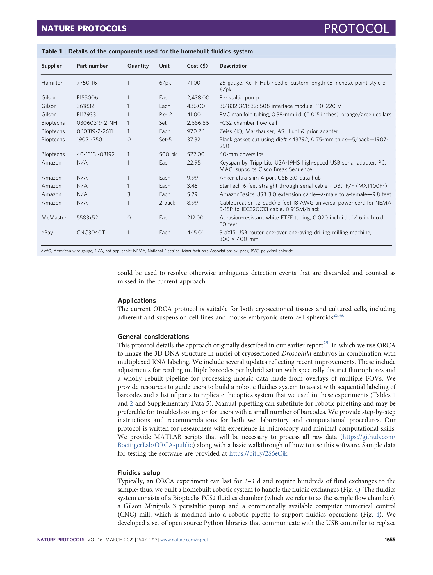
Components for our homebuilt microscope . An EXCEL file containing detailed information - including the supplier(s), part number(s), quantity, units, and total costs - of each component used for our microscope. The total cost of the homebuilt microscope is also included in this table.

Supplementary Data 6

RNA Table . An example of a RNAtable.xlsx file that is used for downstream analysis, such as in BuildMosaicsGUI. See Supplementary Data Legends for full description.

Supplementary Data 7

DNA Table . An example of ExperimentalLayout.xlsx that is used for ChrTracer3 and downstream GUIs. The columns are the same as that of RNAtable.xlsx (see legend for Supplementary Data 6), with two exceptions. 1) For DNA labeling, we typically relabel some of the barcodes at the experiment for quantification purposes. Thus, you will see that at the bottom of the ‘DataType’ column, the last 5 rows are labeled as ‘R’, indicating that these are the barcodes that were relabeled. 2) There is no ‘rnaNames’ column as this is a DNA table.

Supplementary Data 8

ChrTracer3 output file . An example of a fov001_AllFits.csv table that is generated at the end of ChrTracer3 analysis. See Supplementary Data Legends for full description.

Fabrication of angstrom-scale two-dimensional channels for mass transport

Efficient and strand-specific profiling of replicating chromatin with enrichment and sequencing of protein-associated nascent DNA in mammalian cells

The eINTACT method for studying nuclear changes in host plant cells targeted by bacterial effectors in native infection contexts

Rapid reaction optimization by robust and economical quantitative benchtop19F NMR spectroscopy

Profiling native pulmonary basement membrane stiffness using atomic force microscopy

Photoimmunotechnology as a powerful biological tool for molecular-based elimination of target cells and microbes, including bacteria, fungi and viruses

Measuring key human carbohydrate digestive enzyme activities using high-performance anion-exchange chromatography with pulsed amperometric detection

Neural cell isolation from adult macaques for high-throughput analyses and neurosphere cultures

Preparation, validation and use of a vasoactive tryptophan-derived hydroperoxide and relevant control compounds

Neuronal subtype-specific growth cone and soma purification from mammalian CNS via fractionation and fluorescent sorting for subcellular analyses and spatial mapping of local transcriptomes and proteomes

查看全部

Sections

Figures

References

Chromatin conformation capture (3C) methods and fluorescent insitu hybridization (FISH) microscopy have been used to investigate the spatial organization of the genome. Although powerful, both techniques have limitations. Hi-C is challenging for low cell
Introduction
Materials
Procedure
Troubleshooting
Timing
Anticipated results
References
ACKNOWLEDGMENTS

Amano, T. et al. Chromosomal dynamics at the Shh locus: limb bud-specific differential regulation of competence and active transcription. Dev. Cell 16, 47–57 (2009).
Fabre, P. J. et al. Nanoscale spatial organization of the HoxD gene cluster in distinct transcriptional states. Proc. Natl Acad. Sci. USA 112, 13964–13969 (2015).
Williamson, I., Lettice, L. A., Hill, R. E. & Bickmore, W. A. Shh and ZRS enhancer colocalisation is specific to the zone of polarising activity. Development 143, 2994–3001 (2016).
Barbieri, M. et al. Active and poised promoter states drive folding of the extended HoxB locus in mouse embryonic stem cells. Nat. Struct. Mol. Biol. 24, 515–524 (2017).
Fraser, J., Williamson, I., Bickmore, W. A. & Dostie, J. An overview of genome organization and how we got there: from FISH to Hi-C. Microbiol. Mol. Biol. Rev. 79, 347–372 (2015).
Rust, M. J., Bates, M. & Zhuang, X. Sub-diffraction-limit imaging by stochastic optical reconstruction microscopy (STORM). Nat. Methods 3, 793–795 (2006).
Huang, B., Wang, W., Bates, M. & Zhuang, X. Three-dimensional super-resolution imaging by stochastic optical reconstruction microscopy. Science 319, 810–813 (2008).
Beliveau, B. J. et al. Single-molecule super-resolution imaging of chromosomes and in situ haplotype visualization using Oligopaint FISH probes. Nat. Commun. 6, 7147 (2015).
Boettiger, A. N. et al. Super-resolution imaging reveals distinct chromatin folding for different epigenetic states. Nature 529, 418–422 (2016).
Kundu, S. et al. Polycomb repressive complex 1 generates discrete compacted domains that change during differentiation. Mol. Cell 65, 432–446.e5 (2017).
Szabo, Q. et al. TADs are 3D structural units of higher-order chromosome organization in Drosophila. Sci. Adv. 4, eaar8082 (2018).
Kieffer-Kwon, K.-R. et al. Myc regulates chromatin decompaction and nuclear architecture during B cell activation. Mol. Cell 67, 566–578.e10 (2017).
Rao, S. S. P. et al. Cohesin loss eliminates all loop domains. Cell 171, 305–320.e24 (2017).
Huang, P. et al. Comparative analysis of three-dimensional chromosomal architecture identifies a novel fetal hemoglobin regulatory element. Genes Devel. 31, 1704–1713 (2017).
Hsu, S. C. et al. The BET protein BRD2 cooperates with CTCF to enforce transcriptional and architectural boundaries. Mol. Cell 66, 102–116.e7 (2017).
Brown, J. M. et al. A tissue-specific self-interacting chromatin domain forms independently of enhancer-promoter interactions. Nat. Commun. 9, 3849 (2018).
van Bemmel, J. G. et al. The bipartite TAD organization of the X-inactivation center ensures opposing developmental regulation of Tsix and Xist. Nat. Genet. 51, 1024–1034 (2019).
Williamson, I. et al. Developmentally regulated Shh expression is robust to TAD perturbations. Development https://doi.org/10.1242/dev.179523 (2019).
Dixon, J. R. et al. Topological domains in mammalian genomes identified by analysis of chromatin interactions. Nature 485, 376–380 (2012).
Nora, E. P. et al. Spatial partitioning of the regulatory landscape of the X-inactivation centre. Nature 485, 381–385 (2012).
Nora, E. P. et al. Targeted degradation of CTCF decouples local insulation of chromosome domains from genomic compartmentalization. Cell 169, 930–944.e22 (2017).
Schwarzer, W. et al. Two independent modes of chromatin organization revealed by cohesin removal. Nature 551, 51–56 (2017).
Symmons, O. et al. The Shh topological domain facilitates the action of remote enhancers by reducing the effects of genomic distances. Dev. Cell 39, 529–543 (2016).
Finn, E. H. & Misteli, T. Molecular basis and biological function of variability in spatial genome organization. Science 365, eaaw9498 (2019).
Mateo, L. J. et al. Visualizing DNA folding and RNA in embryos at single-cell resolution. Nature 568, 49–54 (2019).
Lubeck, E. & Cai, L. Single-cell systems biology by super-resolution imaging and combinatorial labeling. Nat. Methods 9, 743–748 (2012).
Lubeck, E., Coskun, A. F., Zhiyentayev, T., Ahmad, M. & Cai, L. Single-cell in situ RNA profiling by sequential hybridization. Nat. Methods 11, 360–361 (2014).
Chen, K. H., Boettiger, A. N., Moffitt, J. R., Wang, S. & Zhuang, X. Spatially resolved, highly multiplexed RNA profiling in single cells. Science 348, 412 (2015).
Fazal, F. M. et al. Atlas of subcellular RNA localization revealed by APEX-Seq. Cell 178, 473–490.e26 (2019).
Levsky, J. M., Shenoy, S. M., Pezo, R. C. & Singer, R. H. Single-cell gene expression profiling. Science 297, 836–840 (2002).
Levesque, M. J. & Raj, A. Single-chromosome transcriptional profiling reveals chromosomal gene expression regulation. Nat. Methods 10, 246–248 (2013).
Raj, A., van den Bogaard, P., Rifkin, S. A., van Oudenaarden, A. & Tyagi, S. Imaging individual mRNA molecules using multiple singly labeled probes. Nat. Methods 5, 877–879 (2008).
Beliveau, B. J. et al. Versatile design and synthesis platform for visualizing genomes with Oligopaint FISH probes. Proc. Natl Acad. Sci. USA 109, 21301–21306 (2012).
Moffitt, J. R. et al. High-throughput single-cell gene-expression profiling with multiplexed error-robust fluorescence in situ hybridization. Proc. Natl Acad. Sci. USA 113, 11046–11051 (2016).
Beliveau, B. J. et al. In situ super-resolution imaging of genomic DNA with OligoSTORM and OligoDNA-PAINT. Methods Mol. Biol. 1663, 231–252 (2017).
Beliveau, B. J. et al. OligoMiner provides a rapid, flexible environment for the design of genome-scale oligonucleotide in situ hybridization probes. Proc. Natl Acad. Sci. USA 115, E2183–E2192 (2018).
Jungmann, R. et al. Multiplexed 3D cellular super-resolution imaging with DNA-PAINT and Exchange-PAINT. Nat. Methods https://doi.org/10.1038/nmeth.2835 (2014).
Gelali, E. et al. iFISH is a publically available resource enabling versatile DNA FISH to study genome architecture. Nat. Commun. 10, 1636 (2019).
Boettiger, A. & Murphy, S. Advances in chromatin imaging at kilobase-scale resolution. Trends Genet. 36, 273–287 (2020).
Buxbaum, A. R., Wu, B. & Singer, R. H. Single β-actin mRNA detection in neurons reveals a mechanism for regulating its translatability. Science 343, 419–422 (2014).
Zenklusen, D., Larson, D. R. & Singer, R. H. Single-RNA counting reveals alternative modes of gene expression in yeast. Nat. Struct. Mol. Biol. 15, 1263–1271 (2008).
Paré, A. et al. Visualization of individual Scr mRNAs during Drosophila embryogenesis yields evidence for transcriptional bursting. Curr. Biol. 19, 2037–2042 (2009).
Boettiger, A. N. & Levine, M. Rapid transcription fosters coordinate snail expression in the Drosophila embryo. Cell Rep 3, 8–15 (2013).
Trcek, T. et al. Single-mRNA counting using fluorescent in situ hybridization in budding yeast. Nat. Protoc. 7, 408–419 (2012).
Rouhanifard, S. H. et al. ClampFISH detects individual nucleic acid molecules using click chemistry-based amplification. Nat. Biotechnol. https://doi.org/10.1038/nbt.4286 (2018).
Lyubimova, A. et al. Single-molecule mRNA detection and counting in mammalian tissue. Nat. Protoc. 8, 1743–1758 (2013).
Bintu, B. et al. Super-resolution chromatin tracing reveals domains and cooperative interactions in single cells. Science 362, eaau1783 (2018).
Weber, C. M., Hafner, A., Braun, S. M. G., Boettiger, A. N. & Crabtree, G. R. mSWI/SNF promotes distal repression by titrating polycomb dosage. Preprint at bioRxiv https://doi.org/10.1101/2020.01.29.925586 (2020).
Quinodoz, S. A. et al. Higher-order inter-chromosomal hubs shape 3D genome organization in the nucleus. Cell 174, P744–757.E24 (2018).
Beagrie, R. A. et al. Complex multi-enhancer contacts captured by genome architecture mapping. Nature https://doi.org/10.1038/nature21411 (2017).
McCord, R. P., Kaplan, N. & Giorgetti, L. Chromosome Conformation Capture and Beyond: Toward an Integrative View of Chromosome Structure and Function. Mol. Cell 77, 688–708 (2020).
Nagano, T. et al. Single-cell Hi-C reveals cell-to-cell variability in chromosome structure. Nature 502, 59–64 (2013).
Stevens, T. J. et al. 3D structures of individual mammalian genomes studied by single-cell Hi-C. Nature 544, 59–64 (2017).
Flyamer, I. M. et al. Single-nucleus Hi-C reveals unique chromatin reorganization at oocyte-to-zygote transition. Nature 544, 110–114 (2017).
Gassler, J. et al. A mechanism of cohesin-dependent loop extrusion organizes zygotic genome architecture. EMBO J. 36, 3600–3618 (2017).
Tan, L., Xing, D., Chang, C.-H., Li, H. & Xie, X. S. Three-dimensional genome structures of single diploid human cells. Science 361, 924–928 (2018).
Ramani, V. et al. Massively multiplex single-cell Hi-C. Nat. Methods 14, 263–266 (2017).
Nir, G. et al. Walking along chromosomes with super-resolution imaging, contact maps, and integrative modeling. PLoS Genet. 14, e1007872 (2018).
Beliveau, B. J. et al. In situ super-resolution imaging of genomic DNA with OligoSTORM and OligoDNA-PAINT. Methods Mol. Biol. 1663, 231–252 (2017).
Georgieva, M. et al. Nanometer resolved single-molecule colocalization of nuclear factors by two-color super resolution microscopy imaging. Methods 105, 44–55 (2016).
Wang, S. et al. Spatial organization of chromatin domains and compartments in single chromosomes. Science 353, 598–602 (2016).
Finn, E. H. et al. Extensive heterogeneity and intrinsic variation in spatial genome organization. Cell 176, 1502–1515.e10 (2019).
Cardozo Gizzi, A. M. et al. Microscopy-based chromosome conformation capture enables simultaneous visualization of genome organization and transcription in intact organisms. Mol. Cell 74, 212–222.e5 (2019).
Cardozo Gizzi, A. M. et al. Direct and simultaneous observation of transcription and chromosome architecture in single cells with Hi-M. Nat. Protoc. 15, 840–876 (2020).
Moffitt, J. R. et al. High-performance multiplexed fluorescence in situ hybridization in culture and tissue with matrix imprinting and clearing. Proc. Natl Acad. Sci. USA 113, 14456–14461 (2016).
Eng, C.-H. L. et al. Transcriptome-scale super-resolved imaging in tissues by RNA seqFISH. Nature https://doi.org/10.1038/s41586-019-1049-y (2019).
Magaraki, A., Loda, A., Gribnau, J. & Baarends, W. M. Simultaneous RNA-DNA FISH in mouse preimplantation embryos. Methods Mol. Biol. 1861, 131–147 (2018).
Lai, L.-T., Meng, Z., Shao, F. & Zhang, L.-F. in Long Non-Coding RNAs: Methods and Protocols (eds. Feng, Y. & Zhang, L.) 135–145 (Springer, 2016).
Lanzuolo, C., Roure, V., Dekker, J., Bantignies, F. & Orlando, V. Polycomb response elements mediate the formation of chromosome higher-order structures in the bithorax complex. Nat. Cell Biol. 9, 1167–1174 (2007).
Lee, J. T., Strauss, W. M., Dausman, J. A. & Jaenisch, R. A 450 kb transgene displays properties of the mammalian X-inactivation center. Cell 86, 83–94 (1996).
Deng, W., Shi, X., Tjian, R., Lionnet, T. & Singer, R. H. CASFISH: CRISPR/Cas9-mediated in situ labeling of genomic loci in fixed cells. Proc. Natl Acad. Sci. USA https://doi.org/10.1073/pnas.1515692112 (2015).
Solovei, I. et al. Spatial preservation of nuclear chromatin architecture during three-dimensional fluorescence in situ hybridization (3D-FISH). Exp. Cell Res. 276, 10–23 (2002).
Su, J.-H., Zheng, P., Kinrot, S. S., Bintu, B. & Zhuang, X. Genome-scale imaging of the 3D organization and transcriptional activity of chromatin. Cell https://doi.org/10.1016/j.cell.2020.07.032 (2020).
Rasnik, I., McKinney, S. A. & Ha, T. Nonblinking and long-lasting single-molecule fluorescence imaging. Nat. Methods 3, 891–893 (2006).
Shi, X., Lim, J. & Ha, T. Acidification of the oxygen scavenging system in single-molecule fluorescence studies: in situ sensing with a ratiometric dual-emission probe. Anal. Chem. 82, 6132–6138 (2010).
Tokunaga, M., Imamoto, N. & Sakata-Sogawa, K. Highly inclined thin illumination enables clear single-molecule imaging in cells. Nat. Methods 5, 159–161 (2008).
Lim, D., Ford, T. N., Chu, K. K. & Mertz, J. Optically sectioned in vivo imaging with speckle illumination HiLo microscopy. J. Biomed. Opt. 16, 016014 (2011).
Babcock, H. et al. ZhuangLab/storm-control: v2019.06.28 release. https://doi.org/10.5281/zenodo.3264857 (2019).
Rao, S. S. P. et al. A 3D map of the human genome at kilobase resolution reveals principles of chromatin looping. Cell 159, 1665–1680 (2014).

Tracing DNA paths and RNA profiles in cultured cells and tissues with ORCA

Extended

Supplementary information

推荐阅读