RCPA: An Open-Source R Package for Data Processing, Differential Analysis, Consensus Pathway Analysis, and Visualization
Hung Nguyen, Hung Nguyen, Ha Nguyen, Ha Nguyen, Zeynab Maghsoudi, Zeynab Maghsoudi, Bang Tran, Bang Tran, Sorin Draghici, Sorin Draghici, Tin Nguyen, Tin Nguyen
Abstract
Identifying impacted pathways is important because it provides insights into the biology underlying conditions beyond the detection of differentially expressed genes. Because of the importance of such analysis, more than 100 pathway analysis methods have been developed thus far. Despite the availability of many methods, it is challenging for biomedical researchers to learn and properly perform pathway analysis. First, the sheer number of methods makes it challenging to learn and choose the correct method for a given experiment. Second, computational methods require users to be savvy with coding syntax, and comfortable with command-line environments, areas that are unfamiliar to most life scientists. Third, as learning tools and computational methods are typically implemented only for a few species (i.e., human and some model organisms), it is difficult to perform pathway analysis on other species that are not included in many of the current pathway analysis tools. Finally, existing pathway tools do not allow researchers to combine, compare, and contrast the results of different methods and experiments for both hypothesis testing and analysis purposes. To address these challenges, we developed an open-source R package for Consensus Pathway Analysis (RCPA) that allows researchers to conveniently: (1) download and process data from NCBI GEO; (2) perform differential analysis using established techniques developed for both microarray and sequencing data; (3) perform both gene set enrichment, as well as topology-based pathway analysis using different methods that seek to answer different research hypotheses; (4) combine methods and datasets to find consensus results; and (5) visualize analysis results and explore significantly impacted pathways across multiple analyses. This protocol provides many example code snippets with detailed explanations and supports the analysis of more than 1000 species, two pathway databases, three differential analysis techniques, eight pathway analysis tools, six meta-analysis methods, and two consensus analysis techniques. The package is freely available on the CRAN repository. © 2024 The Authors. Current Protocols published by Wiley Periodicals LLC.
Basic Protocol 1 : Processing Affymetrix microarrays
Basic Protocol 2 : Processing Agilent microarrays
Support Protocol : Processing RNA sequencing (RNA-Seq) data
Basic Protocol 3 : Differential analysis of microarray data (Affymetrix and Agilent)
Basic Protocol 4 : Differential analysis of RNA-Seq data
Basic Protocol 5 : Gene set enrichment analysis
Basic Protocol 6 : Topology-based (TB) pathway analysis
Basic Protocol 7 : Data integration and visualization
INTRODUCTION
Together with the ability to generate a large amount of data, high-throughput technologies have also brought the challenge of translating such data into biological knowledge. Regardless of the laboratory technology being used, a comparative study (e.g., disease vs healthy) typically yields a set of genes or proteins that are differentially expressed (DE) between the two phenotypes. Though important, these lists of DE genes do not explain the mechanisms involved in the underlying conditions by themselves. To translate DE genes into biological knowledge, researchers have developed knowledge bases that capture the knowledge about the function, location and other properties of the genes and gene products. One of the first such knowledge bases was the Gene Ontology (GO) (The Gene Ontology Consortium, 2021). GO consists of a controlled vocabulary of terms that describe biological processes, cellular locations, and biochemical functions, as well as the relationships between them. These together form an ontology. Furthermore, GO also provides associations between genes and these terms, thus capturing the knowledge about the gene functions and localization within the cell.
As soon as such annotations started to become available, analysis methods were developed to take advantage of them. The first analysis approach was the over-representation analysis (ORA) that identifies the gene sets, e.g., GO terms, which are enriched in differentially expressed (DE) genes (Beissbarth & Speed, 2004; Hosack et al., 2003; Khatri et al., 2002). The drawbacks of ORA approaches include that they: (1) only consider the number of DE genes and ignore the actual expression changes, and (2) assume that genes are independent, which is not true. Functional Class Scoring (FCS) approaches have been developed to address these drawbacks. These include the GSEA family of methods (Efron & Tibshirani, 2007; Mootha et al., 2003; Subramanian et al., 2005). The main improvement is that these approaches can identify situations in which small but coordinated changes in the expression of functionally related genes are important.
While GO captures the associations between genes and various biological processes, cellular locations, and biochemical functions, it does not provide any direct information about the interactions between the genes and/or gene products. Basically, each GO term can be seen as an unordered, unstructured set of genes that are associated with it. The next step was taken by trying to describe the complex phenomena that take place in living organisms by describing the various signals and interactions between genes, gene products, and/or metabolites. These are captured in directed graphs that are commonly referred to as pathways. Examples include the Kyoto Encyclopedia of Genes and Genomes (KEGG) (Kanehisa et al., 2017) and Reactome (Croft et al., 2014). Pathways can be further divided into gene signaling pathways and metabolic pathways. In gene signaling pathways, the nodes represent genes, and the edges represent signals or interactions between genes and/or gene products. In a metabolic pathway, nodes represent biochemical molecules and edges represent reactions that take place between such biomolecules. The reactions are carried out by enzymes that are coded by genes so that in a metabolic pathway, genes are associated with the edges rather than the nodes.
Once such sophisticated pathway models have become available, the challenge was to identify those pathways that are important in a given phenotype. The first analysis approaches for pathways were to simply consider the pathways as simple sets of genes and use the methods previously developed for gene set analysis: ORA and FCS. However, ORA and FCS are limited because they do not account for the hierarchical structure of pathways or interactions between genes. Topology-based (TB) approaches were developed to further incorporate knowledge about gene topology and network in their hypothesis testing (Draghici et al., 2007; Tarca et al., 2009). Topology-based approaches are able to consider all important elements ignored by ORA and FCS methods, i.e., the positions and roles of all the genes in every pathway, the direction and type of signals between them, etc. Because of their advantages, many more topology-based approaches have since been proposed (Glaab et al., 2010; Gu et al., 2012; Gu & Wang, 2013; Mitrea et al., 2013; Nguyen, Diaz, et al., 2016; Nguyen et al., 2020).
Despite the availability of many pathway analysis methods, it is tremendously challenging for biomedical researchers to learn and to properly perform pathway analysis. First, the sheer number of methods makes it demanding for scientists to learn and choose the correct method for their experiments. As reported in our previous benchmarking article (Nguyen et al., 2019), there is no single method that is always superior to others. The suitability of a method depends on the research hypothesis users seek to answer. Second, testing available methods requires users to be savvy with coding syntax and comfortable with command-line environments, areas that are unfamiliar to most life scientists. Third, many available tools are typically implemented only for human and a few model organisms, thus making it difficult to perform pathway analysis on hundreds of other species that are not included in current analysis tools. Finally, meta-analysis and consensus analysis are missing from many existing pathway analysis tools. Meta-analysis techniques focus on combining independent but related studies to increase statistical power (Normand, 1999) whereas consensus analysis combines analysis results obtained from methods with different underlying hypotheses for a better understanding of biological mechanisms (Nguyen et al., 2021).
To address the challenges above, we introduce the R package for Consensus Pathway Analysis (RCPA) that implements a complete analysis pipeline, including: (1) downloading and processing data from NCBI Gene Expression Omnibus, (2) performing differential analysis using techniques developed for both microarray and sequencing data, (3) performing systems-level analysis using different methods for enrichment analysis and topology-based (TB) analysis, (4) performing meta-analysis and consensus analysis, and (5) visualizing analysis results and exploring significantly impacted pathways across multiple analyses. The package supports the analysis of >1000 species, two pathway databases, three differential analysis techniques, eight pathway analysis tools, six meta-analysis methods, and two consensus analysis techniques. The package is freely available on the CRAN repository (see Internet Resources).
STRATEGIC PLANNING
Flowchart
Figure 1 shows the analysis workflow implemented in the RCPA package. The full pipeline consists of eight protocols that can be divided into four main modules: (1) data processing (Basic Protocols 1 and 2, and Support Protocol), (2) differential analysis (Basic Protocols 3 and 4), (3) systems-level analysis (Basic Protocols 5 and 6), and (4) integrative analysis (Basic Protocol 7). Each protocol includes established analysis methods and visualization techniques. The pipeline is designed to work with transcriptome data, which can be either the expression data obtained from microarrays or raw read counts obtained from RNA sequencing (RNA-Seq).
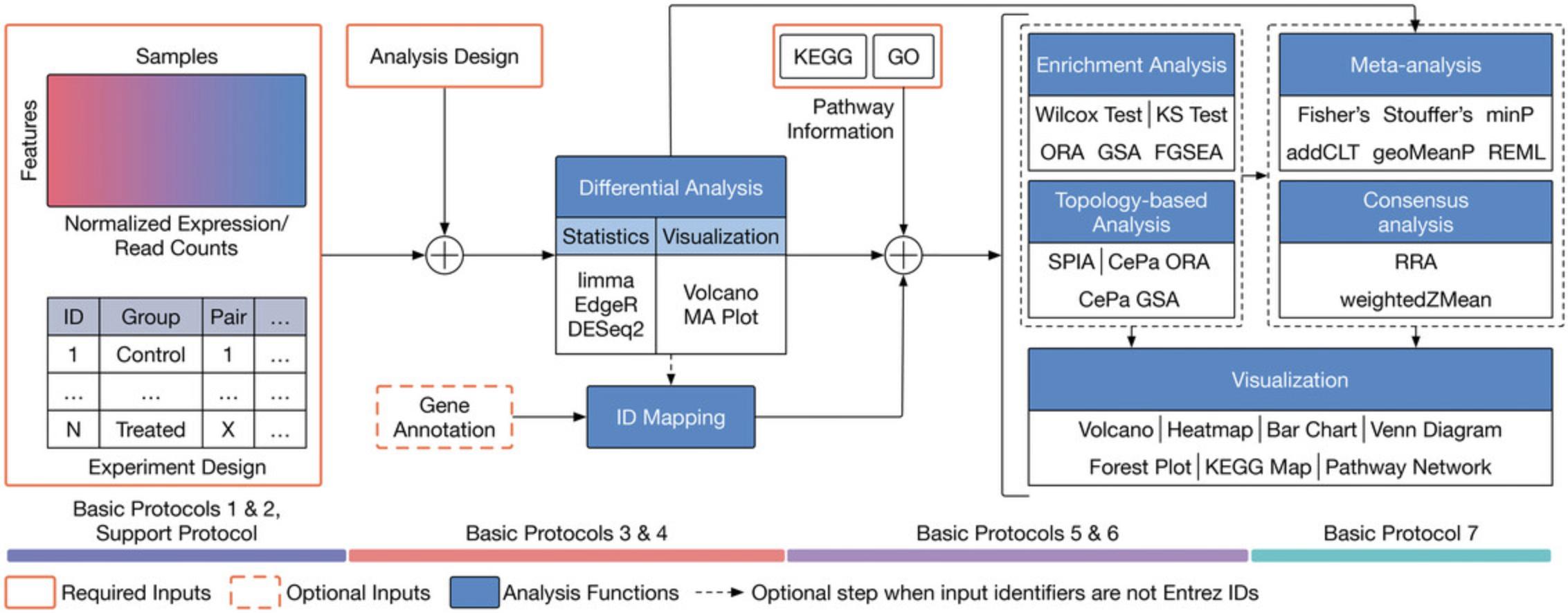
The first module is data processing. We introduce Basic Protocols 1 and 2, and Support Protocol that can process Affymetrix, Agilent, and RNA-Seq, respectively. The output of this module is a SummarizedExperiment object that stores both the expression data and metadata (i.e., sample information, condition, tissue, etc.).
The second module focuses on differential analysis. We introduce Basic Protocols 3 and 4 that provide instructions for performing differential analysis of microarray and RNA-Seq data, respectively. The module includes differential analysis techniques available in limma (Ritchie et al., 2015), DESeq2 (Love et al., 2014), and edgeR (Robinson et al., 2010). The input of the module is the SummarizedExperiment object obtained from the first module. The output is a SummarizedExperiment object that includes both the input (expression and metadata) and the differential analysis results.
The third module focuses on systems-level analysis. We introduce Basic Protocols 5 and 6 for gene set enrichment analysis and topology-based (TB) pathway analysis, respectively. The main difference between gene set enrichment and TB pathway analysis is that the former treats each pathway as a set of genes, whereas the latter considers gene interactions and pathway topology. Basic Protocol 5 covers five gene set enrichment analysis techniques: the Wilcoxon test (Wilcoxon, 1992), the Kolmogorov-Smirnov (KS) test (Massey Jr, 1951), over-representation analysis (ORA) (Huang et al., 2009; Khatri et al., 2002), fast gene set enrichment analysis (FGSEA) (Korotkevich et al., 2021; Sergushichev, 2016), and gene set analysis (GSA) (Efron & Tibshirani, 2007). Basic Protocol 6 covers three TB pathway analysis methods: signaling pathway impact analysis (SPIA) (Draghici et al., 2007; Tarca et al., 2009), centrality-based pathway enrichment for ORA extension (CePa ORA), and for GSA extension (CePa GSA) (Gu et al., 2012; Gu & Wang, 2013). The input of the third module is the SummarizedExperiment object obtained from the second module. The output is a data frame that includes the systems-level analysis results.
The fourth module focuses on integrative analysis. We introduce Basic Protocol 7 for meta-analysis and consensus analysis. Meta-analysis includes a range of techniques to integrate independent but related datasets to increase statistical power and accuracy. Meta-analysis can be performed at both gene and pathway levels to find robust sets of differentially expressed genes and impacted pathways. In contrast, the main objective of consensus pathway analysis is to allow users to see the differences, as well as the consensus results across many methods that rely on distinctively different hypotheses. Consensus analysis can also be extended to compare multiple experiments and computational methods at the same time, so that users can compare different hypotheses, experimental designs, and technologies. The package includes six meta-analysis methods to combine p -values and statistics across independent datasets: Fisher's method (Fisher, 1925), Stouffer's method (Stouffer et al., 1949), addCLT (Nguyen et al., 2017; Nguyen, Tagett, et al., 2016), minimum p -value (Tippett, 1931), geometric mean (Vovk & Wang, 2020), and restricted maximum likelihood (REML) (Viechtbauer, 2005). The package also implements two methods for consensus analysis: robust rank aggregation (RRA) (Kolde et al., 2012) for combining pathway ranks, and weighted mean for combining z-values obtained from multiple analyses.
QuickStart
Throughout the eight protocols in this article, we consistently use three datasets of three data platforms (GSE5281 of Affymetrix, GSE61196 of Agilent, and GSE153873 of RNA-Seq) in our examples. The data and analysis results of all three datasets are pre-saved by the package and this allows users to skip any protocol. For example, users can go directly to Basic Protocol 7 and perform data visualization without executing any code from the preceding protocols. They only need to call the function RCPA::loadData() to load the results from the preceding protocols before running the code in visualization. We also include the code for RCPA::loadData() to load necessary data at the beginning of each protocol.
For the convenience of readers, we also created Table 1 to list all data objects obtained from each protocol. The first column of the table shows the names of the objects, while the second column explains the content of each object. Users can load any of the above objects using the function RCPA::loadData(). For example, users can simply use affyDEExperiment <- RCPA::loadData(“affyDEExperiment”) to load the differential analysis results of the Affymetrix dataset GSE5281 stored in the object affyDEExperiment. The availability of pre-saved data objects would allow users to test any of the eight protocols without the need of going through the preceding protocols. Note that the objects of Basic Protocol 7 (Data Integration and Visualization) are not listed here because it is the last protocol described in this article, and its data objects are not used in any other protocols. We also organized all code snippets in this article into a single Jupyter notebook, and it is freely available on GitHub (see Internet Resources).
| Object name | Description |
|---|---|
| Basic Protocol 1: Processing Affymetrix data | |
| affyDataset | Affymetrix dataset GSE5281 after pre-processing and normalization |
| Basic Protocol 2: Processing Agilent data | |
| agilDataset | Agilent dataset GSE61196 after pre-processing and normalization |
| Support Protocol: Processing RNA-Seq data | |
| RNASeqDataset | RNA-Seq dataset GSE153873 after pre-processing and normalization |
| Basic Protocol 3: Differential analysis of microarray data | |
| affyDEExperiment | Differential analysis results of the Affymetrix dataset GSE5281 |
| agilDEExperiment | Differential analysis results of the Agilent dataset GSE61196 |
| Basic Protocol 4: Differential analysis of RNA-Seq data | |
| RNASeqDEExperiment | Differential analysis results of the RNA-Seq dataset GSE153873 |
| Basic Protocol 5: Gene set enrichment analysis | |
| KEGGGenesets | Gene sets downloaded from KEGG |
| GOTerms | GO terms downloaded from Gene Ontology (GO) |
| affyKSResult | Enrichment results of the Affymetrix dataset GSE5281 using KS test |
| affyWilcoxResult | Enrichment results of the Affymetrix dataset GSE5281 using Wilcoxon test |
| affyORAResult | Enrichment results of the Affymetrix dataset GSE5281 using ORA |
| affyFGSEAResult | Enrichment results of the Affymetrix dataset GSE5281 using FGSEA |
| affyGSAResult | Enrichment results of the Affymetrix dataset GSE5281 using GSA |
| agilKSResult | Enrichment results of the Agilent dataset GSE61196 using KS test |
| agilWilcoxResult | Enrichment results of the Agilent dataset GSE61196 using Wilcoxon test |
| agilORAResult | Enrichment results of the Agilent dataset GSE61196 using ORA |
| agilFGSEAResult | Enrichment results of the Agilent dataset GSE61196 using FGSEA |
| agilGSAResult | Enrichment results of the Agilent dataset GSE61196 using GSA |
| RNASeqKSResult | Enrichment results of the RNA-Seq dataset GSE153873 using KS test |
| RNASeqWilcoxResult | Enrichment results of the RNA-Seq dataset GSE153873 using Wilcoxon test |
| RNASeqORAResult | Enrichment results of the RNA-Seq dataset GSE153873 using ORA |
| RNASeqFGSEAResult | Enrichment results of the RNA-Seq dataset GSE153873 using FGSEA |
| RNASeqGSAResult | Enrichment results of the RNA-Seq dataset GSE153873 using GSA |
| Basic Protocol 6: Topology-based (TB) pathway analysis | |
| SPIANetwork | KEGG pathway graphs for TP analysis using SPIA |
| CePaNetwork | KEGG pathway graphs for TP analysis using CePa ORA and CePa GSA |
| affySPIAResult | TB pathway analysis results of the Affymetrix dataset GSE5281 using SPIA |
| affyCePaORAResult | TB pathway analysis results of the Affymetrix dataset GSE5281 using CePa ORA |
| affyCePaGSAResult | TB pathway analysis results of the Affymetrix dataset GSE5281 using CePa GSA |
| agilSPIAResult | TB pathway analysis results of the Agilent dataset GSE61196 using SPIA |
| agilCePaORAResult | TB pathway analysis results of the Agilent dataset GSE61196 using CePa ORA |
| agilCePaGSAResult | TB pathway analysis results of the Agilent dataset GSE61196 using CePa GSA |
| RNASeqSPIAResult | TB pathway analysis results of the RNA-Seq dataset GSE153873 using SPIA |
| RNASeqCePaORAResult | TB pathway analysis results of the RNA-Seq dataset GSE153873 using CePa ORA |
| RNASeqCePaGSAResult | TB pathway analysis results of the RNA-Seq dataset GSE153873 using CePa GSA |
- a Users can load any of the above objects using the function RCPA::loadData(). For example, users can use affyDEExperiment <- RCPA::loadData(“affyDEExperiment”) to load the differential analysis results of the Affymetrix dataset GSE5281 stored in the object affyDEExperiment. Note that the objects of Basic Protocol 7 (Data Integration and Visualization) are not listed here because it is the last protocol, and its data objects are not used in any other protocols.
Basic Protocol 1: PROCESSING AFFYMETRIX MICROARRAYS
Basic Protocol 1 guides users through the process of converting raw CEL files into a SummarizedExperiment object, which is a data structure designed for efficient downstream analysis. There are three main steps in this protocol: (1) preparing the CEL files and sample information file, (2) processing the CEL files to obtain the expression data, and (3) creating the SummarizedExperiment object.
Necessary Resources
Hardware
- An internet-connected computer or laptop with at least 8 GB of RAM and 20 GB of free hard drive space
Software
- R runtime environment (version 4.0.0 or later)
- RCPA package from the CRAN repository (see Internet Resources)
- This can be done by simply executing the following command in the R console: install.packages("RCPA")
Files
- A list of CEL.gz files
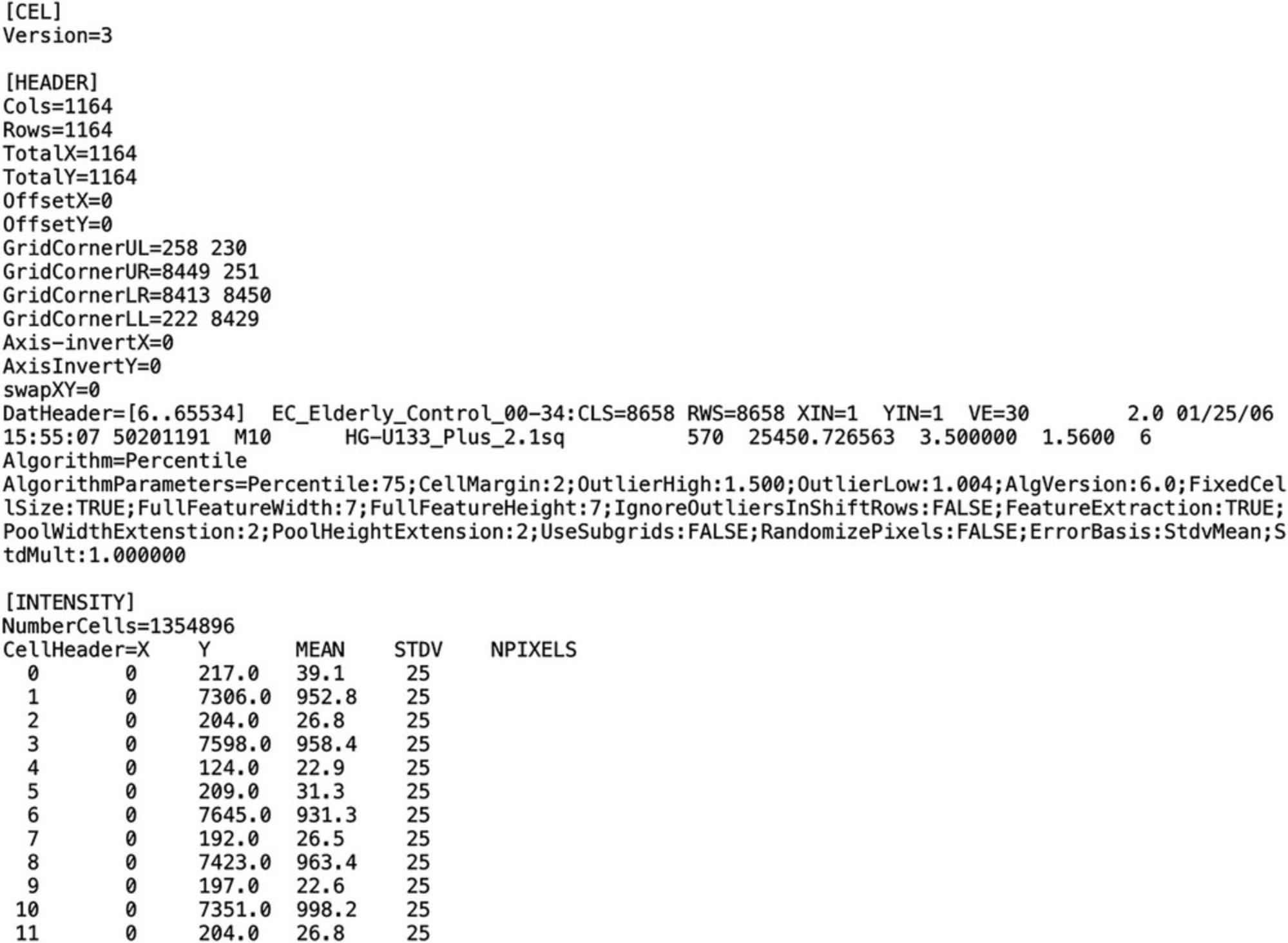
CEL files are the raw data files generated by Affymetrix microarray scanners. The .gz extension indicates that the files are compressed using the gzip program. The raw content of the CEL files can be read by any text editor. Figure 2 shows an example CEL file. In this protocol, the example CEL files used for analysis will be downloaded from the GEO dataset with the accession number GSE5281.
- A spreadsheet containing sample information in CSV or TSV format
In this spreadsheet, each row represents a sample, and each column represents its attribute, e.g., sample ID, disease status, tissue, etc. In this protocol, we will create the example spreadsheet by extracting the sample information from the GEO dataset GSE5281.
Preparing the CEL files and sample information file
To proceed with the data processing, users need to organize all CEL files in a single folder. In the following example, we will download the CEL files from the GEO dataset GSE5281 using the downloadGEO() function implemented in the RCPA package. If users already have the CEL files, they can skip this step and go directly to the next step.
1.Create a local directory to save the data:
- userPath <- tempdir() # or user-defined directory path
downloadPath <- file.path(userPath, "GSE5281")
if(!dir.exists(downloadPath)) dir.create(downloadPath)
2.Browse and search for the underlying dataset on the GEO website.
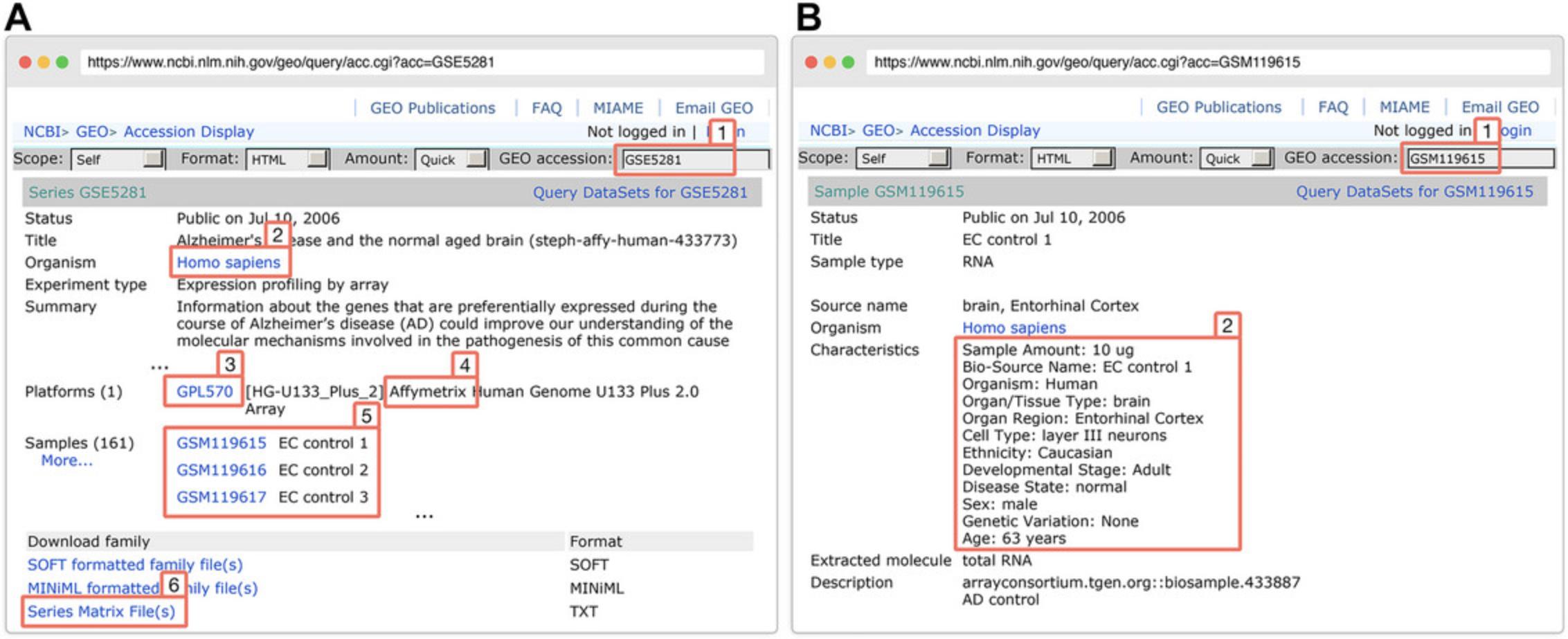
3.Download the Affymetrix dataset from GEO using the function downloadGEO():
-
download the data
downloadedFiles <- RCPA::downloadGEO(GEOID = "GSE5281", platform = "GPL570", protocol = "affymetrix", destDir = downloadPath)
-
display the list of downloaded files
print(head(downloadedFiles))
-
console output
[1] "metadata.csv" "GSM119615.CEL.gz" "GSM119616.CEL.gz" "GSM119617.CEL.gz"
[5] "GSM119618.CEL.gz" "GSM119619.CEL.gz"
Reading sample information and processing CEL files
4.Read the sample information from the metadata file:
-
read the metadata file
affySampleInfo <- read.csv(file.path(downloadPath, "metadata.csv"))
-
Display the metadata
print(head(affySampleInfo[, c("geo_accession", "characteristics_ch1.4","characteristics_ch1.8")]))
-
console output
| geo_accession | characteristics_ch1.4 | characteristics_ch1.8 |
| GSM119615 | Organ Region: Entorhinal | Cortex Disease State: normal |
| GSM119616 | Organ Region: Entorhinal | Cortex Disease State: normal |
| GSM119617 | Organ Region: Entorhinal | Cortex Disease State: normal |
| GSM119618 | Organ Region: Entorhinal | Cortex Disease State: normal |
| GSM119619 | Organ Region: Entorhinal | Cortex Disease State: normal |
| GSM119620 | Organ Region: Entorhinal | Cortex Disease State: normal |
5.Process the CEL files and obtain the expression matrix:
-
read the CEL files
affyExprs <- RCPA::processAffymetrix(dir = downloadPath, samples = affySampleInfo$geo_accession)
-
display the expression matrix
print(head(affyExprs, c(5, 6)))
-
console output
| GSM119615 | GSM119616 | GSM119617 | GSM119618 | GSM119619 | GSM119620 | |
| 1007_s_at | 3.043234 | 3.055157 | 3.144277 | 3.150378 | 3.084336 | 2.989966 |
| 1053_at | 1.698974 | 1.645050 | 1.618537 | 1.589216 | 1.676278 | 1.581733 |
| 117_at | 1.795751 | 1.770719 | 1.805597 | 1.995794 | 1.688068 | 1.961556 |
| 121_at | 2.553174 | 2.668456 | 2.801450 | 2.784216 | 2.588638 | 2.692849 |
| 1255_g_at | 1.626691 | 1.940055 | 1.663162 | 1.483875 | 2.354096 | 1.671216 |
Creating the SummarizedExperiment object
We will store the processed data in a SummarizedExperiment object, which is an S4 data object defined by the SummarizedExperiment package. The SummarizedExperiment object allows users to perform unified operations, e.g., add or remove samples, for both the metadata and assay. It thereby ensures that the metadata and observational data remain in sync, mitigating the risk of data mishandling that might occur when manually processing expression data and metadata.
6.Check that the required package is installed:
-
load the SummarizedExperiment package
library(SummarizedExperiment)
7.Create the SummarizedExperiment object:
-
create the SummarizedExperiment object
affyDataset <- SummarizedExperiment::SummarizedExperiment(assays = affyExprs, colData = affySampleInfo)
-
display the SummarizedExperiment object
print(affyDataset)
-
console output
class: SummarizedExperiment
dim: 54675 161
metadata(0):
assays(1): ‘’
rownames(54675): 1007_s_at 1053_at … AFFX-r2-P1-cre-3_at
AFFX-r2-P1-cre-5_at
rowData names(0):
colnames(161): GSM119615 GSM119616 … GSM238955 GSM238963
colData names(71): X title … sample.amount.ch1 sex.ch1
8.Access the expression data and sample information stored in SummarizedExperiment object:
-
access expression data
-
affyExprs <- SummarizedExperiment::assay(affyDataset)
-
display affyExprs
-
print(head(affyExprs, c(5, 6)))
-
console output
| GSM119615 | GSM119616 | GSM119617 | GSM119618 | GSM119619 | GSM119620 | |
| 1007_s_at | 3.043234 | 3.055157 | 3.144277 | 3.150378 | 3.084336 | 2.989966 |
| 1053_at | 1.698974 | 1.645050 | 1.618537 | 1.589216 | 1.676278 | 1.581733 |
| 117_at | 1.795751 | 1.770719 | 1.805597 | 1.995794 | 1.688068 | 1.961556 |
| 121_at | 2.553174 | 2.668456 | 2.801450 | 2.784216 | 2.588638 | 2.692849 |
| 1255_g_at | 1.626691 | 1.940055 | 1.663162 | 1.483875 | 2.354096 | 1.671216 |
-
Access to sample information
-
affySampleInfo <- SummarizedExperiment::colData(affyDataset)
-
display affySampleInfo
-
head(affySampleInfo[, c("title", "characteristics_ch1.4", "characteristics_ch1.8")])
-
console output
|
|
|
|
|
|
|
|
|
|
|
|
|
|
|
|
|
|
|
|
|
Basic Protocol 2: PROCESSING AGILENT MICROARRAYS
This Basic Protocol guides users through the process of converting raw Agilent TXT files into a SummarizedExperiment object. Similar to Basic Protocol 1, there are three main steps in this protocol: (1) preparing the TXT files and sample information file, (2) processing the TXT files to obtain the expression data, and (3) creating the SummarizedExperiment object.
Necessary Resources
Hardware
- An internet-connected computer or laptop with at least 8 GB of RAM and 20 GB of free hard drive
Software
- R runtime environment (version 4.0.0 or later)
- RCPA package from the CRAN repository
Files
- A list of TXT.gz files
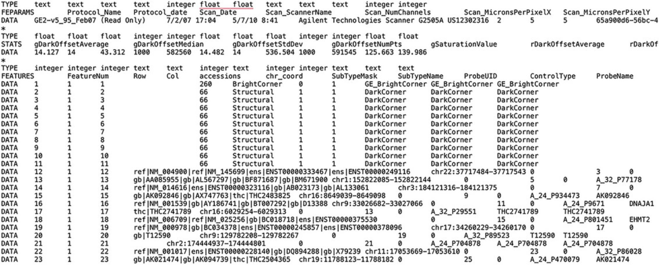
The TXT files here are the raw data files generated by Agilent microarray scanners as Agilent does not use any file extension for its raw data files. These TXT files can be read by any text editor. Figure 4 shows an example TXT file for Agilent. In this protocol, the example TXT files used for analysis will be downloaded from the GEO dataset with the accession number GSE61196.
- A spreadsheet containing sample information in CSV or TSV format
In this spreadsheet, each row represents a sample, and each column represents its attribute, e.g., sample ID, disease status, tissue, etc. In this protocol, we will create the example spreadsheet by extracting the sample information from the GEO dataset GSE61196.
Preparing the TXT files and sample information file
Similar to Basic Protocol 1, users need to organize all TXT files in a single folder. In the following example, we will download the TXT files from the GEO dataset GSE61196 using the downloadGEO() function implemented in the RCPA package. If users already have the TXT files, they can skip this step and go directly to the next step.
1.Create a local directory to save the downloaded data:
- userPath <- tempdir() # or user-defined directory path
downloadPath <- file.path(userPath, "GSE61196")
if(!dir.exists(downloadPath)) dir.create(downloadPath)
2.Browse and search for the dataset on NCBI GEO.
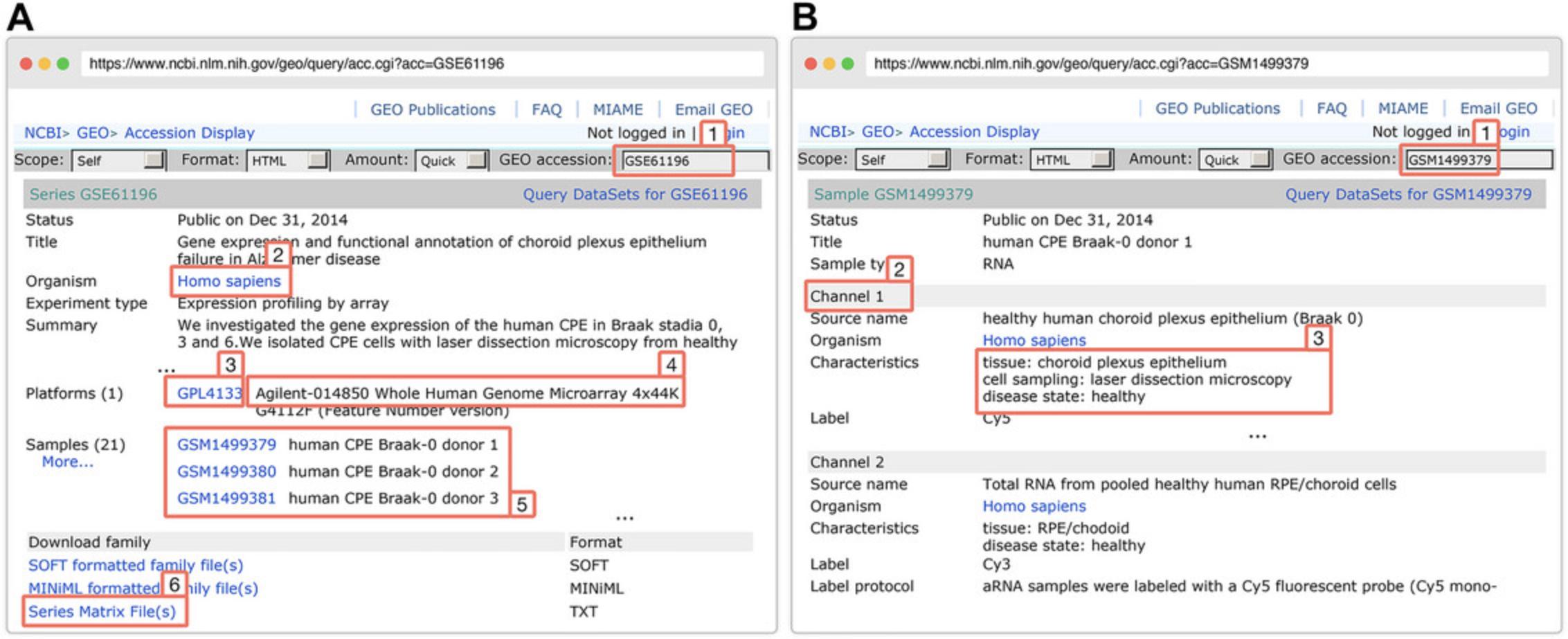
3.Download the Agilent data using the downloadGEO() function:
-
download the data
downloadedFiles <- RCPA::downloadGEO(GEOID = "GSE61196", platform = "GPL4133", protocol = "agilent", destDir = downloadPath)
-
display the list of downloaded files
head(downloadedFiles)
-
console output
[1] "metadata.csv" "GSM1499379.TXT.gz" "GSM1499380.TXT.gz"
[4] "GSM1499381.TXT.gz" "GSM1499382.TXT.gz" "GSM1499383.TXT.gz"
Reading sample information and processing Agilent TXT files
4.Read the sample information from the metadata file:
-
read the metadata file
agilSampleInfo <- read.csv(file.path(downloadPath, "metadata.csv"))
-
Display the metadata
print(agilSampleInfo[9:14, c("geo_accession", "characteristics_ch2.1", "tissue.ch2")])
-
console output
|
|
|
|
|
|
|
|
|
|
|
|
|
|
|
|
|
|
|
|
|
5.Process the TXT files and obtain the expression matrix:
-
read the TXT files
agilExprs <- RCPA::processAgilent(dir = downloadPath, samples = agilSampleInfo$geo_accession, greenOnly = FALSE)
-
display the expression matrix
print(agilExprs[9:14, 1:6])
-
console output
|
|
|
|
|
|
|
|
|
|
|
|
|
|
|
|
|
|
|
|
|
|
|
|
|
|
|
|
|
|
|
|
|
|
|
|
|
|
|
|
|
|
|
|
|
|
|
|
|
|
Creating the SummarizedExperiment object
6.Create the SummarizedExperiment object:
-
create the SummarizedExperiment object
agilDataset <- SummarizedExperiment::SummarizedExperiment(assays = agilExprs, colData = agilSampleInfo)
-
display the SummarizedExperiment object
print(agilDataset)
-
console output
class: SummarizedExperiment
dim: 45015 21
metadata(0):
assays(1): ''
rownames(45015): GE_BrightCorner DarkCorner … GE_BrightCorner
GE_BrightCorner
rowData names(0):
colnames(21): GSM1499379 GSM1499380 … GSM1499398 GSM1499399
colData names(49): X title … tissue.ch1 tissue.ch2
7.Access the expression data and sample information stored in SummarizedExperiment object:
-
Access expression data
-
agilExprs <- SummarizedExperiment::assay(agilDataset)
-
Display agilExprs
-
print(agilExprs[9:14, 1:6])
-
Console output
|
|
|
|
|
|
|
|
|
|
|
|
|
|
|
|
|
|
|
|
|
|
|
|
|
|
|
|
|
|
|
|
|
|
|
|
|
|
|
|
|
|
|
|
|
|
|
|
|
-
Access sample information
-
agilSampleInfo <- SummarizedExperiment::colData(agilDataset)
-
Display agilSampleInfo
-
print(agilSampleInfo[9:14, c("geo_accession", "characteristics_ch2.1", "tissue.ch2")])
-
Console output
|
|
|
|
|
|
|
|
|
|
|
|
|
|
|
|
|
|
|
|
|
|
|
|
|
|
|
|
|
Support Protocol: PROCESSING RNA SEQUENCING (RNA-Seq) DATA
This Support Protocol guides users through the process of converting a raw count matrix file into a SummarizedExperiment object. There are two main steps in this protocol: (1) preparing the count matrix file and sample information file, and (2) creating the SummarizedExperiment object.
Necessary Resources
Hardware
- An internet-connected computer or laptop with at least 8 GB of RAM and 20 GB of free hard drive space
Software
- R runtime environment (version 4.0.0 or later)
- RCPA package from the CRAN repository
Files
- A count matrix file
The count matrix file is a table that contains the raw read counts for each gene in each sample. The count matrix file can be saved in any format, e.g., TXT, CSV, TSV, etc., depending on what data processing pipeline users use to generate the count matrix file. We recommend that users follow the best practices for data processing and normalization specific to each RNA-Seq technology (Conesa et al., 2016; Robertson et al., 2010). Figure 6 shows an example count matrix. In this protocol, we will download the count matrix file from the GEO dataset with the accession number GSE153873.
- A spreadsheet containing sample information, CSV or TSV format
In this spreadsheet, each row represents a sample, and each column represents its attribute, e.g., sample ID, disease status, tissue, etc. In this protocol, we will create the example spreadsheet by extracting the sample information from the GEO dataset GSE153873.
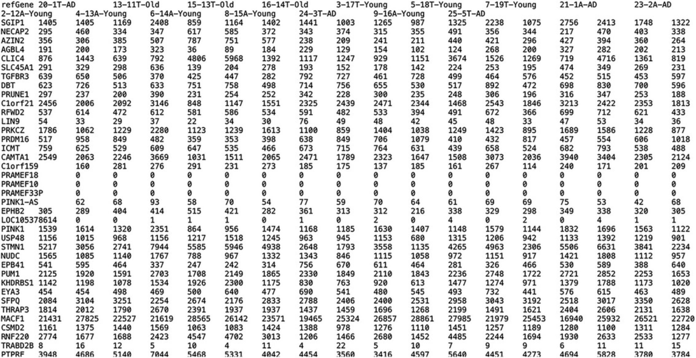
Preparing the count matrix file and sample information file
Users can skip this step if they already have the count matrix file and sample information file. In this protocol, we will create the sample information file by extracting the sample information from the GEO dataset GSE153873 using the getGEO() function implemented in the GEOquery package. We will also download the count matrix file from the GEO dataset GSE153873 using the getGEOSuppFiles() function.
1.Browse and search for the RNA-Seq dataset on GEO:
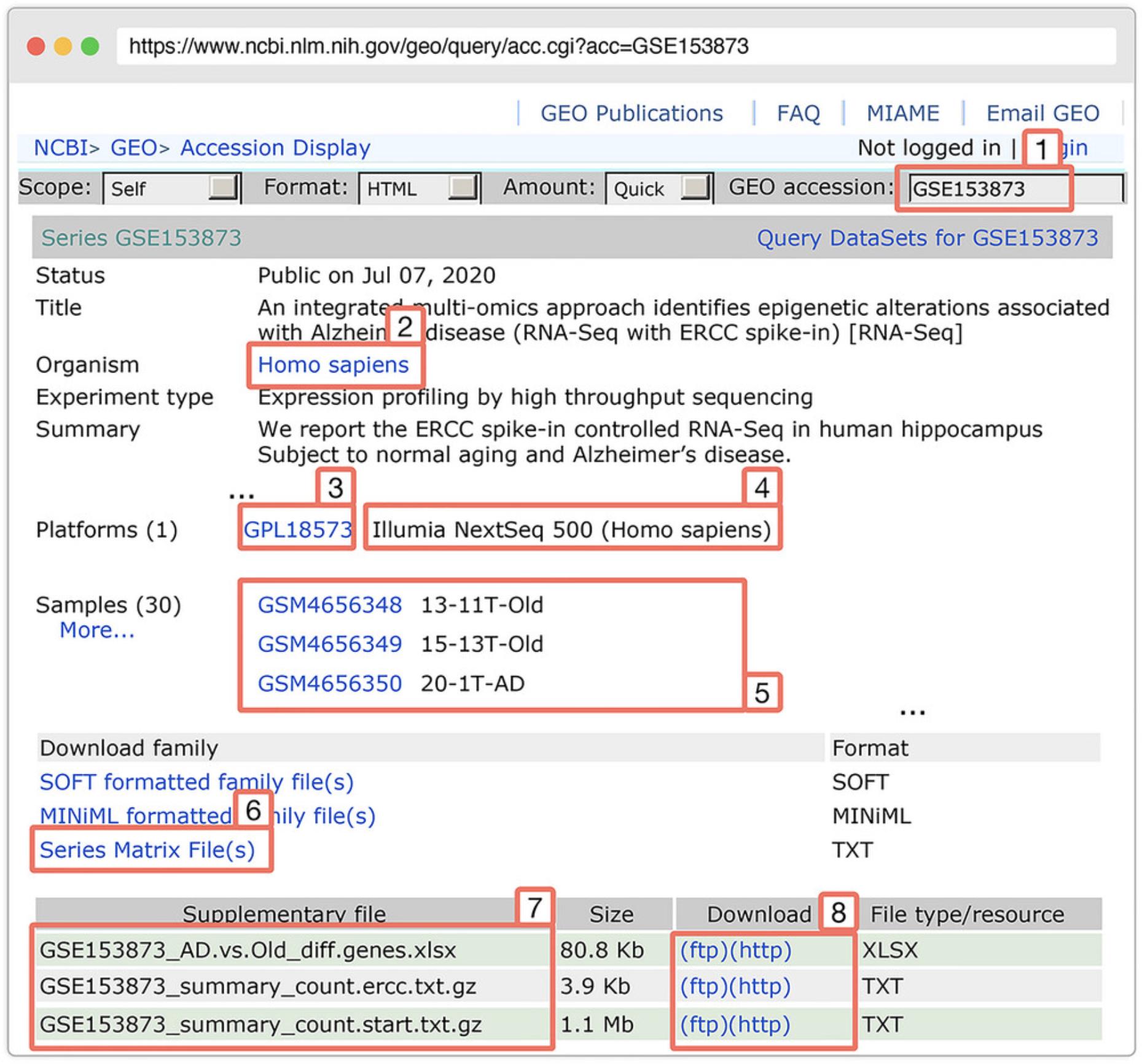
2.Create a local directory to save the downloaded data:
- userPath <- tempdir() # or user-defined directory path
downloadPath <- file.path(userPath, "GSE153873")
if(!dir.exists(downloadPath)) dir.create(downloadPath)
3.Get the sample information from the GEO dataset:
-
Download the GEO object to get metadata
GEOObject <- GEOquery::getGEO(GEO = "GSE153873", GSEMatrix = T, getGPL = F, destdir = downloadPath)
-
Check the length of GEOObject
message("length: ", length(GEOObject))
-
console output
length: 1
-
Extract the dataset from the GEOObject
samplesData <- GEOObject[[1]]
-
Export sample data
metadata <- Biobase::pData(samplesData)
-
save the metadata for later use
write.csv(metadata, file.path(downloadPath, "metadata.csv"))
-
preview the metadata
print(head(metadata[, c("title", "status", "characteristics_ch1.1")]))
-
console output
|
|
|
|
|
|
|
|
|
|
|
|
|
|
|
|
|
|
|
|
|
|
|
|
|
|
|
|
|
4.Download the raw count data from the GEO dataset:
-
Download the supplementary files
GEOquery::getGEOSuppFiles(GEO = "GSE153873", fetch_files = TRUE, baseDir = userPath)
-
Check the downloaded data files
list.files(file.path(userPath, "GSE153873"))
-
Console output
[1] "GSE153873_AD.vs.Old_diff.genes.xlsx" "GSE153873_summary_count.ercc.txt.gz"
[3] "GSE153873_summary_count.star.txt.gz"
Creating the SummarizedExperiment object
5.Examine the format of the count matrix file:
-
read the first 10 lines of the count matrix file
countsFile <- file.path(userPath, "GSE153873", "GSE153873_summary_count.star.txt.gz")
lines <- readLines(countsFile, n = 10)
-
display the first 50 characters of each line
print(substr(lines, start = 1, stop = 50))
-
console output
|
|
|
|
|
|
|
|
|
|
|
|
|
|
|
|
|
|
|
|
6.Read the sample information and count matrix file:
-
read the previously saved metadata
RNASeqSampleInfo <- read.csv(file.path(downloadPath, "metadata.csv"))
-
read the count matrix file
countsData <- read.table(countsFile, header = TRUE, sep = "\t", fill = 0, row.names = 1, check.names = FALSE)
-
preview the metadata and count matrix
print(head(RNASeqSampleInfo[, c("title", "status", "characteristics_ch1.1")], 3))
print(head(countsData, c(3,6)))
-
console output
metadata
|
|
|
|
|
|
|
|
|
|
|
|
|
|
|
|
|
-
count matrix
|
|
|
|
|
|
|
|
|
|
|
|
|
|
|
|
|
|
|
|
|
|
|
|
|
|
|
|
|
7.Rename the column names of the count matrix:
-
Get the sample titles
sampleTitles <- RNASeqSampleInfo$title
-
Rearrange the column of the count matrix
countsData <- countsData[, sampleTitles]
-
Rename the column names
colnames(countsData) <- rownames(RNASeqSampleInfo)
-
Preview the count matrix
print(head(countsData, c(5,6)))
-
console output
|
|
|
|
|
|
|
|
|
|
|
|
|
|
|
|
|
|
|
|
|
|
|
|
|
|
|
|
|
|
|
|
|
|
|
|
|
|
|
|
|
|
|
8.Create the SummarizedExperiment object:
-
RNASeqDataset <- SummarizedExperiment::SummarizedExperiment(assays = as.matrix(countsData), colData = metadata)
-
Display the SummarizedExperiment object
print(RNASeqDataset)
-
Console output
class: SummarizedExperiment
dim: 27135 30
metadata(0):
assays(1): ''
rownames(27135): SGIP1 NECAP2 … KIR2DS1 KIR2DL5B
rowData names(0):
colnames(30): GSM4656348 GSM4656349 … GSM4656376 GSM4656377
colData names(38): title geo_accession … disease state:ch1 tissue:ch1
9.Access the expression data and sample information stored in SummarizedExperiment object:
-
Access the expression data:
RNASeqExprs <- SummarizedExperiment::assay(RNASeqDataset)
-
Display RNASeqExprs
head(RNASeqExprs, c(5, 6))
-
Console output:
|
|
|
|
|
|
|
|
|
|
|
|
|
|
|
|
|
|
|
|
|
|
|
|
|
|
|
|
|
|
|
|
|
|
|
|
|
|
|
|
|
|
|
-
Access to the sample information data
RNASeqSampleInfo <- SummarizedExperiment::colData(RNASeqDataset)
-
Display RNASeqSampleInfo
print(RNASeqSampleInfo[1:5, c("characteristics_ch1", "characteristics_ch1.1", "diseasestate:ch1")])
-
Console output:
DataFrame with 5 rows and 3 columns
|
|
|
|
|
|
|
|
|
|
|
|
|
|
|
|
|
|
|
|
|
|
|
|
|
Basic Protocol 3: DIFFERENTIAL ANALYSIS OF MICROARRAY DATA (AFFYMETRIX AND AGILENT)
Differential expression analysis is a fundamental analysis that aims to identify genes that are differentially expressed between distinct conditions or phenotypes. The analysis of Affymetrix and Agilent only differs in data processing and normalization. After the processing step, their downstream analysis procedures are the same. There are many popular excellent techniques that can be used for differential analysis (Kerr et al., 2000; Love et al., 2014; Student, 1908). In this article, we choose to describe three basic methods that have been widely used in the field, namely limma (Ritchie et al., 2015), DESeq2 (Love et al., 2014), and edgeR (Robinson et al., 2010). Note that limma is often applied for continuous data (microarray expression, or normalized RNA-Seq expression, e.g., RPKM, TPM, etc.) whereas DESeq2 and edgeR are often used for read counts (positive integers).
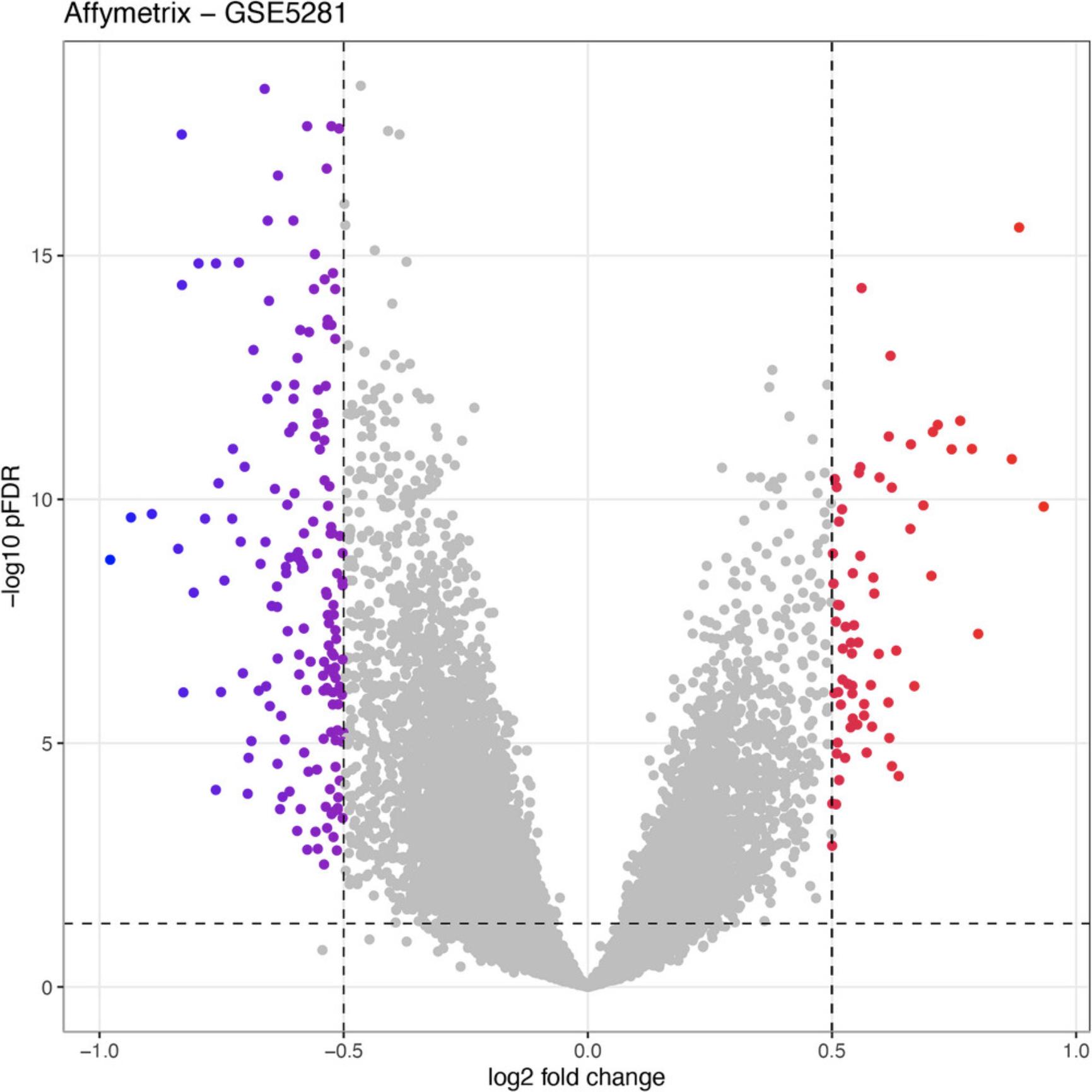
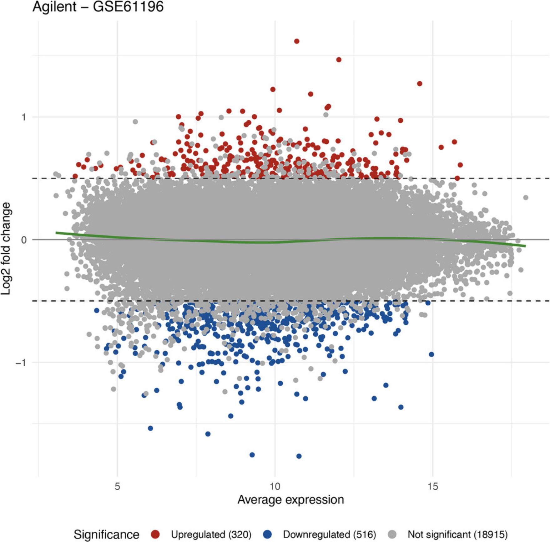
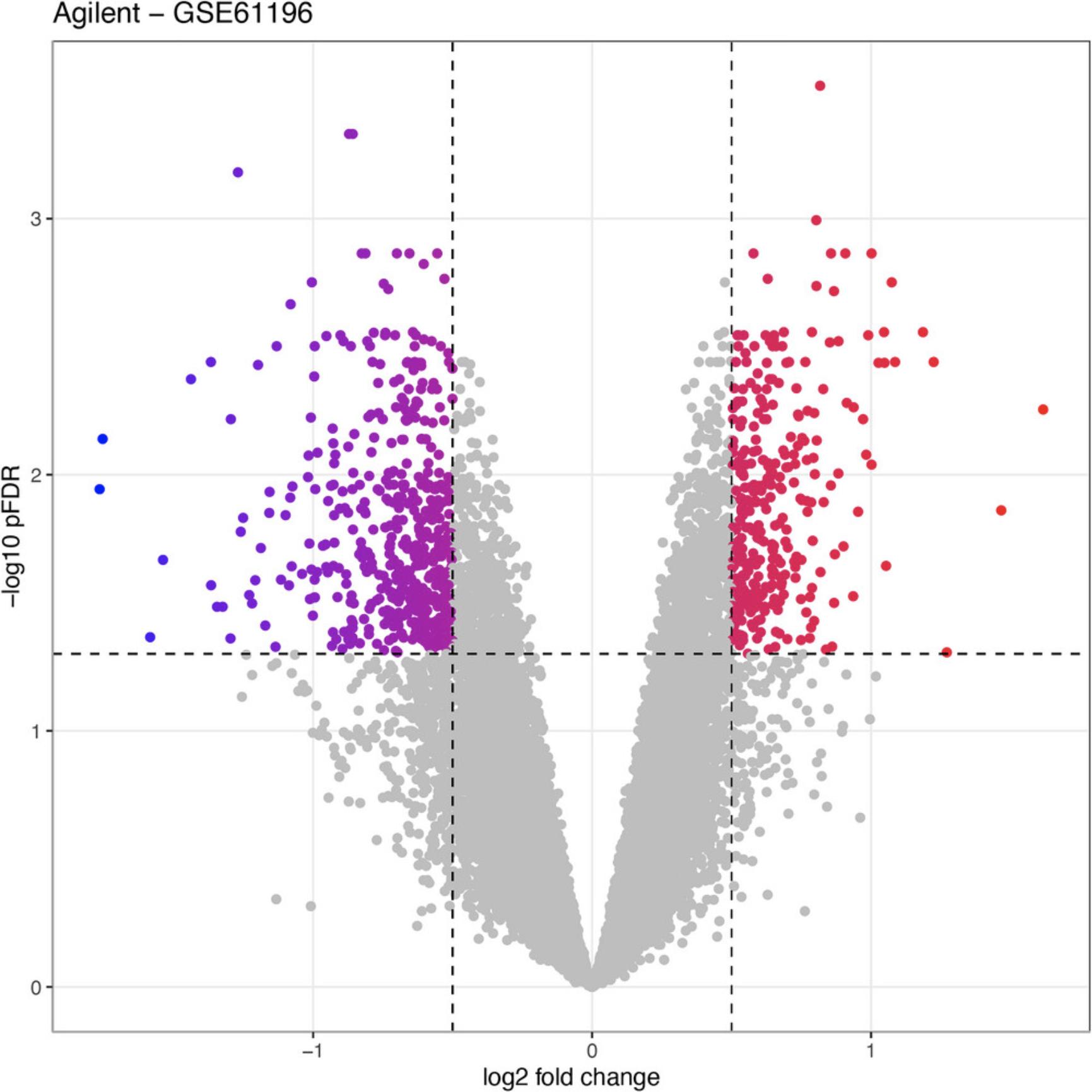
In this protocol, we introduce the function runDEAnalysis() that applies limma (Ritchie et al., 2015) for differential expression analysis, specifically designed for microarray data. The procedure involves several key steps, including the definition and representation of experimental design using design and contrast matrices. This is followed by the conversion of probe IDs into Entrez gene IDs, which will be used for subsequent analysis. Additionally, we offer two visualization functions, plotMA() and plotVolcanoDE(), that are designed to enhance the visualization of the differential analysis results. Visualization is a common practice to examine the results of differential analysis before users proceed with pathway analysis and data integration.
Here, we provide step-and-step guidelines on differential analysis of the two microarray datasets (GSE5281 and GSE61196) that have been used thus far. Note that after data processing, as described in Basic Protocols 1 and 2, we have the SummarizedExperiment objects that include expression data and sample metadata.
Necessary Resources
Hardware
- An internet-connected computer or laptop with at least 8 GB of RAM and 20 GB of free hard drive space
Software
- R runtime environment (version 4.0.0 or later)
- RCPA package from the CRAN repository (see Internet Resources)
Besides the functions in RCPA, we will need to use the functions in the SummarizedExperiment to access the data stored in the SummarizedExperiment object. Similarly, some functions from the ggplot2 package will be used to add the title or modify the figures generated by the plot functions in RCPA. We can ensure the required packages are installed by loading them as shown in the following code snippet:
- library(RCPA)
- library(SummarizedExperiment)
- library(ggplot2)
Files
- A SummarizedExperiment object
A SummarizedExperiment object has at least two attributes: (1) assays, storing the expression data matrix, in which rows are genes/transcripts and columns are samples; and (2) colData, storing a data frame containing the sample information. Users can refer to Basic Protocols 1 and 2 for more information about the SummarizedExperiment object.
- A gene mapping data frame
A gene mapping data frame has two columns: (2) FROM, containing the genes/transcript IDs currently used in the assay data; and (2) TO, containing the corresponding Entrez IDs. Users need to manually prepare this data frame and can save it as .rda, .rds, .txt, or .csv files, or other formats. Consequently, they will use the appropriate R functions to load the file. We will guide users on how to prepare this data frame in our practical example below.
- Sample files
Users can use function RCPA::loadData() to load the pre-saved Microarray datasets obtained from Basic Protocols 1 and 2 from our GitHub repository (https://github.com/tinnlab/RCPA/tree/main/.data). The first step in this protocol will guide the user in loading the pre-saved data using the function.
Affymetrix: GSE5281
1.If users skipped Basic Protocol 1, they could use RCPA::loadData() to load the data:
-
Load the Affymetrix data processed in Basic Protocol 1
affyDataset <- RCPA::loadData("affyDataset")
2.Create a design matrix for differential analysis:
-
Read metadata from the SummarizedExperiment object named affyDataset
affySampleInfo <- SummarizedExperiment::colData(affyDataset)
-
Add a column specifying the condition of each sample (normal or Alzheimer's)
affySampleInfo
-
Factorize the new column
affySampleInfo
-
Add a new column to specify the region of the sample tissue,
use make.names() to remove special characters and
use tolower() to make all characters lowercase
affySampleInfo
affySampleInfo
-
Factorize the newly added column
affySampleInfo
-
Update the affyDataset object
SummarizedExperiment::colData(affyDataset) <- affySampleInfo
-
Create a design matrix
affyDesign <- model.matrix(∼0 + condition + region + condition:region, data = affySampleInfo)
-
Remove special characters in column names
colnames(affyDesign) <- make.names(colnames(affyDesign))
The samples of the GSE5281 dataset fall into two conditions, “normal” and “Alzheimer's,” which are specified in the characteristics_ch1.8 column. Each sample is also associated with a specific brain region, such as the entorhinal cortex, hippocampus, primary visual cortex, and so on, denoted in the characteristics_ch1.4 column. Consequently, both attributes serve as experimental variables within the design matrix.
The initial step in the code snippet involves the addition of two new columns that represent the sample's condition and the associated brain region to the sample information that is stored in the returned SummarizedExperiment object described in Basic Protocol 1.These new columns are essentially cleaner versions of the original characteristics_ch1.8 and characteristics_ch1.4 columns. The original columns are often manually curated and may contain special characters or duplicated data, which could potentially lead to errors in the analysis. Therefore, it is crucial to perform data cleaning before proceeding with any further steps. Users can verify the updated sample information by executing the following command line:
-
Check update
affyDataset
-
Console output:
class: SummarizedExperiment
dim: 54675 161
metadata(0):
assays(1): ''
rownames(54675): 1007_s_at 1053_at … AFFX-TrpnX-5_at AFFX-TrpnX-M_at
rowData names(0):
colnames(161): GSM119615 GSM119616 … GSM238955 GSM238963
colData names(72): title geo_accession … condition region
The above code shows that the new columns condition and region were added to the affyDataset object, as indicated in the final row of the console (i.e., under “colData names”). To generate the design matrix, we introduce the function model.matrix(), sourced from the built-in R package called stats. Utilizing this function entails providing two essential pieces of information: a formula resembling a regression model, such as ∼var1 + var2, and the dataset containing the variables referenced in this formula. Here, in the above snippet, the formula “∼0 + condition + region + condition:region ” defines the design matrix to include the main effects of condition and region, as well as the interaction between condition and region. The term ∼0 indicates that the intercept should not be included in the design matrix since the intercept is not of interest in the analysis. By following the snippet, users can observe the example of the design matrix as it appears in the following console output:
-
print the design matrix
print(affyDesign[1:5, 1:3])
-
Console output
|
|
|
|
|
|
|
|
|
|
|
|
|
|
|
|
|
|
|
|
|
|
|
|
|
3.Create a contrast matrix for differential analysis:
-
Create a contrast matrix
affyContrast <- limma::makeContrasts(conditionalzheimer-conditionnormal,levels = affyDesign)
-
print contrast
head(affyContrast)
-
Console output
|
|
|
|
|
|
|
|
|
|
|
|
|
|
|
|
4.Perform differential analysis using the function runDEAnalysis():
-
Run differential expression analysis
affyDEExperiment <- RCPA::runDEAnalysis(affyDataset, method = "limma", design = affyDesign, contrast = affyContrast, annotation = "GPL570")
-
Display affyDEExperiment
affyDEExperiment
-
Console output
class: SummarizedExperiment
dim: 21367 161
metadata(4): DEAnalysis.method DEAnalysis.design DEAnalysis.contrast DEAnalysis.mapping
assays(1): counts
rownames(21367): 55101 92840 … 9695 83887
rowData names(9): PROBEID ID … sampleSize pFDR
colnames(161): GSM119615 GSM119616 … GSM238955 GSM238963
colData names(72): title geo_accession … condition region
5.Access to the differential expression analysis result stored in the SummarizedExperiment object:
-
Extract the differential analysis result
affyDEResults <- SummarizedExperiment::rowData(affyDEExperiment)
-
Print in R console
head(affyDEResults, c(3,5))
-
console output
DataFrame with 3 rows and 5 columns
|
|
|
|
|
|
|
|
|
|
|
|
|
|
|
|
|
|
|
|
|
|
|
|
|
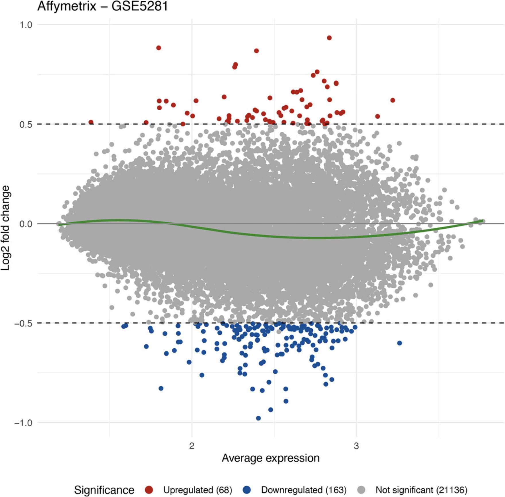
6.Visualize the differential analysis results using MA plot:
-
Visualize the differential analysis results using MA plot
RCPA::plotMA(affyDEResults, logFCThreshold = 0.5) +
ggplot2::ggtitle("Affymetrix - GSE5281")
7.Visualize the differential analysis results using volcano plot:
-
Visualize the differential analysis results using volcano plot
RCPA::plotVolcanoDE(affyDEResults, logFCThreshold = 0.5) +
ggplot2::ggtitle("Affymetrix - GSE5281")
Agilent: GSE61196
The analysis of Agilent datasets is similar to that of Affymetrix datasets. Users can use the following snippets to perform differential expression analysis for Agilent datasets.
8.If users skipped Basic Protocol 2, they can use RCPA::loadData() to load the data:
-
Load the Agilent data processed in Basic Protocol 2
agilDataset <- RCPA::loadData("agilDataset")
9.Create a design matrix and a contrast matrix:
-
Access to the sample information data
agilSampleInfo <- SummarizedExperiment::colData(agilDataset)
-
Add a column specifying the condition of the sample,
which can be either normal or alzheimer
agilSampleConditions <- ifelse(grepl("healthy", agilSampleInfo$source_name_ch1),"normal", "alzheimer")
-
Factorize the newly added column
agilSampleInfo$condition <- factor(agilSampleConditions)
-
Update the colData attribute with new column
SummarizedExperiment::colData(agilDataset) <- agilSampleInfo
-
Create a design matrix
agilDesign <- model.matrix(∼0 + condition, data = SummarizedExperiment::colData(agilDataset))
-
Create a contrast matrix
agilContrast <- limma::makeContrasts("conditionalzheimer-conditionnormal", levels = agilDesign)
10.Retrieve the platform information and its gene annotation from GEO database:
-
Download the information for GPL4133 platform:
GPL4133Pl <- GEOquery::getGEO(GEO = "GPL4133")
-
Display GPL4133Pl
str(GPL4133Pl)
-
Console output
Formal class 'GPL' [package "GEOquery"] with 2 slots
..@ dataTable:Formal class 'GEODataTable' [package "GEOquery"] with 2 slots
.. .. ..@ columns:'data.frame': 22 obs. of 2 variables:
.. .. .. ..$ Column : chr [1:22] "ID" "COL" "ROW" "NAME" ...
.. .. .. ..$ Description: chr [1:22] "Agilent feature number" "Column" "Row" "NAME" ...
.. .. ..@ table :'data.frame': 45220 obs. of 22 variables:
.. .. .. ..$ ID : int [1:45220] 1 2 3 4 5 6 7 8 9 10 ...
.. .. .. ..$ COL : int [1:45220] 266 266 266 266 266 266 266 266 266 266 ...
.. .. .. ..$ ROW : int [1:45220] 170 168 166 164 162 160 158 156 154 152 ...
.. .. .. ..$ NAME : chr [1:45220] "GE_BrightCorner" "DarkCorner" "DarkCorner" "DarkCorner" ...
.. .. .. ..$ SPOT_ID : chr [1:45220] "GE_BrightCorner" "DarkCorner" "DarkCorner" "DarkCorner"
.. .. .. .. .. .. .. ..
- ..@ header :List of 27
- .. ..$ catalog_number : chr "G4112F"
- .. ..$ contact_city : chr "Palo Alto"
- .. ..$ contact_country : chr "USA"
- .. ..$ contact_email : chr "cag_sales-na@agilent.com"
- .. ..$ contact_institute : chr "Agilent Technologies"
- .. ..[output truncated] .. ..
In the above code, we use getGEO() from the GEO query package to obtain the platform from GEO. When using this function, users need to provide the platform ID to the GEO parameter. In this example, we set GEO as “GPL4133”. The function returns an object of “GPL” class, and we assign the result to GPL4133Pl variable. Next, users can use the built-in function str() to examine the data structure of this object, as shown in the example code. From the console output, we can see that the GPL4133Pl variable has 2 slots. The first slot is dataTable that is used to store the gene annotation data, and the second one is header, which is a list containing platform metadata.
-
Access to the dataTable slot in GPL4133Pl:
GPL4133Anno <- GEOquery::dataTable(GPL4133Pl)
-
Display GPLL4133Anno:
str(GPL4133Anno)
-
Console output
Formal class 'GEODataTable' [package "GEOquery"] with 2 slots
..@ columns:'data.frame': 22 obs. of 2 variables:
.. ..$ Column : chr [1:22] "ID" "COL" "ROW" "NAME" ...
.. ..$ Description: chr [1:22] "Agilent feature number" "Column" "Row" "NAME" ...
..@ table :'data.frame': 45220 obs. of 22 variables:
.. ..$ ID : int [1:45220] 1 2 3 4 5 6 7 8 9 10 ...
.. ..$ COL : int [1:45220] 266 266 266 266 266 266 266 266 266 266 ...
.. ..$ ROW : int [1:45220] 170 168 166 164 162 160 158 156 154 152 ...
.. ..$ NAME : chr [1:45220] "GE_BrightCorner" "DarkCorner" "DarkCorner" "DarkCorner" ...
.. ..$ SPOT_ID : chr [1:45220] "GE_BrightCorner" "DarkCorner" "DarkCorner" "DarkCorner" ...
.. ..$ CONTROL_TYPE : chr [1:45220] "pos" "pos" "pos" "pos" ...
.. ..$ REFSEQ : chr [1:45220] "" "" "" "" ...
.. ..$ GB_ACC : chr [1:45220] "" "" "" "" ...
.. ..$ GENE : int [1:45220] NA NA NA NA NA NA NA NA NA NA ...
.. ..$ GENE_SYMBOL : chr [1:45220] "" "" "" "" ...
.. ..$ GENE_NAME : chr [1:45220] "" "" "" "" ...
.. ..$ UNIGENE_ID : chr [1:45220] "" "" "" "" ...
.. ..$ ENSEMBL_ID : chr [1:45220] "" "" "" "" ...
.. ..$ TIGR_ID : chr [1:45220] "" "" "" "" ...
.. ..$ ACCESSION_STRING : chr [1:45220] "" "" "" "" ...
.. ..$ CHROMOSOMAL_LOCATION: chr [1:45220] "" "" "" "" ...
.. ..$ CYTOBAND : chr [1:45220] "" "" "" "" ...
.. ..$ DESCRIPTION : chr [1:45220] "" "" "" "" ...
.. ..$ GO_ID : chr [1:45220] "" "" "" "" ...
.. ..$ SEQUENCE : chr [1:45220] "" "" "" "" ...
.. ..$ SPOT_ID : logi [1:45220] NA NA NA NA NA NA ...
.. ..$ ORDER : int [1:45220] 1 2 3 4 5 6 7 8 9 10 ...
Because the dataTable slot is an object of GEODataTable class from the GEOquery package. Therefore, users can use the function GEOquery::dataTable() to access this slot as shown in the above code. We assign the object returned by this function to GPL4133Anno variable. Users can also use the command str(GPL4133Anno) to further examine the returned object. As in the console output, the GPL4133Anno variable stores two data frames. One of the data frames is stored in the table attribute, in which the columns are spot IDs and their matched gene annotation. The other data frame is stored in columns, which contain the full descriptions of columns in the former data frame.
-
Access to annotation data
GPL4133AnnoTbl <- GEOquery::Table(GPL4133Anno)
-
display annotation
print(GPL4133AnnoTbl[9:14, c("SPOT_ID", "GENE", "GENE_SYMBOL")])
-
Console output
|
|
|
|
|
|
|
|
|
|
|
|
|
|
|
|
|
|
|
|
|
11.Create a mapping data frame that will be used for differential analysis:
-
Create the mapping data frame
GPL4133GeneMapping <- data.frame(FROM = GPL4133AnnoTbl
- #Display GPL4133GeneMapping:
print(GPL4133GeneMapping[15:20,])
-
Console output:
|
|
|
|
|
|
|
|
|
|
|
|
|
|
12.Perform differential analysis using the function runDEAnalysis():
-
Run differential expression analysis
agilDEExperiment <- RCPA::runDEAnalysis(agilDataset, method = “limma”, design = agilDesign, contrast = agilContrast, annotation = GPL4133GeneMapping)
-
Extract the outcome of differential expression analysis
agilDEResults <- SummarizedExperiment::rowData(agilDEExperiment)
-
Print in R console
head(agilDEResults, c(3,5))
-
Console output
DataFrame with 3 rows and 5 columns
|
|
|
|
|
|
|
|
|
|
|
|
|
|
|
|
|
|
|
|
|
|
|
|
|
13.Visualize the results using MA and volcano plots:
-
MA plot
RCPA::plotMA(agilDEResults, logFCThreshold = 0.5) +
ggplot2::ggtitle("Agilent - GSE61196")
-
Volcano plot
RCPA::plotVolcanoDE(agilDEResults, logFCThreshold = 0.5) +
ggplot2::ggtitle("Agilent - GSE61196")
Basic Protocol 4: DIFFERENTIAL ANALYSIS OF RNA-Seq DATA
Users can utilize the same function runDEAnalysis() to perform differential analysis for RNA-Seq data. Users are required to provide the SummarizedExperiment object containing the expression data and sample information, design matrix, contrast matrix, gene IDs mapping, and the differential analysis method. For RNA-Seq data, users can choose from three different methods implemented in RCPA package: “limma”, “DESeq2”, or “EdgeR”. The choice of the differential analysis method depends on how users pre-process and normalize their data. If users want to work with raw count data, then “DESeq2” or “EdgeR” can be employed as the analysis method. In contrast, if users want to work with normalized expression data, such as TPM, FPKM, or RPKM, then they should choose “limma” as the differential analysis method.
In this protocol, we perform differential analysis for the RNA-Seq dataset GSE153873 processed in Support Protocol. We assume that users have already executed the provided code to obtain the SummarizedExperiment object, that contains the raw count data and sample metadata. Here we illustrate the application of runDEAnalysis() for conducting differential expression analysis using RNA-Seq data.
Necessary Resources
Hardware
- An internet-connected computer or laptop with at least 8 GB of RAM and 20 GB of free hard drive space
Software
- R runtime environment (version 4.0.0 or later)
- RCPA package from the CRAN repository (see Internet Resources)
Beside the functions in RCPA, we will need to use the functions in the SummarizedExperiment to access the data stored in the SummarizedExperiment object. Similarly, some functions from the ggplot2 package will be used to add the title or modify the figures generated by the plot functions in RCPA. We can ensure the required packages are installed by loading them as shown in the following code snippet:
- library(RCPA)
- library(SummarizedExperiment)
- library(ggplot2)
Files
- A SummarizedExperiment object
A SummarizedExperiment object that has at least two attributes: (1) assays, storing the expression data matrix, in which rows are genes/transcripts and columns are samples; and (2) colData, storing a data frame containing the sample information. Users can refer to Support Protocol for more information about the object SummarizedExperiment.
- A gene mapping data frame
A gene mapping data frame has two columns: (1) FROM, containing the genes/transcript IDs currently used in the assay data, and (2) TO, containing the corresponding Entrez ID. Users need to manually prepare this data frame and can save it as .rda, .rds, .txt, or .csv files, or other formats. Consequently, they will use the appropriate R functions to load the file. We will guide users on how to prepare this data frame in our practical example below.
- Sample files
Users can use function RCPA::loadData() to load the pre-saved RNA-Seq dataset in Support Protocol from our GitHub repository (https://github.com/tinnlab/RCPA/tree/main/.data). The first step in this protocol will guide the user in loading the pre-saved data using the function.
1.If users skipped Support Protocol, they can use RCPA::loadData() to load the data:
-
Load the RNA-Seq dataset
RNASeqDataset <- RCPA::loadData("RNASeqDataset")
2.Create the design and contrast matrices:
-
Access to the sample information data
RNASeqSampleInfo <- SummarizedExperiment::colData(RNASeqDataset)
-
Add a column specifying the condition of the sample,
which can be either normal or alzheimer
RNASeqSampleConditions <- ifelse(grepl("Alzheimer",RNASeqSampleInfo$characteristics_ch1.1), "alzheimer", "normal")
-
Factorize the newly added column
RNASeqSampleInfo$condition <- factor(RNASeqSampleConditions)
-
Update the colData attribute with new column
SummarizedExperiment::colData(RNASeqDataset) <- RNASeqSampleInfo
-
Create a design matrix
RNASeqDesign <- model.matrix(∼0 + condition, data = SummarizedExperiment::colData(RNASeqDataset))
-
Create a contrast matrix
RNASeqContrast <- limma::makeContrasts("conditionalzheimer-conditionnormal", levels = RNASeqDesign)
3.Define the mapping between the ID of the assay in SummarizedExperiment and Entrez ID:
-
Install the genome-wide annotation database for human
if (!require("BiocManager", quietly = TRUE))
install.packages("BiocManager")
BiocManager::install("org.Hs.eg.db")
-
Load the annotation database
library(org.Hs.eg.db)
-
Get the current gene IDs used in RNA-Seq dataset
RNASeqGeneIDs <- rownames(RNASeqDataset)
-
Create a mapping dataframe
GeneSymbolMapping <- AnnotationDbi::select(x = org.Hs.eg.db, keys = RNASeqGeneIDs,keytype = "SYMBOL",columns = c("SYMBOL", "ENTREZID"))
colnames(GeneSymbolMapping) <- c("FROM", "TO")
-
Print the first 6 rows into R console
head(GeneSymbolMapping)
-
Console output
|
|
|
|
|
|
|
|
|
|
|
|
|
|
|
|
|
|
|
|
|
|
4.Perform differential analysis using the function runDEAnalysis():
-
Perform differential analysis
RNASeqDEExperiment <- RCPA::runDEAnalysis(RNASeqDataset, method = "DESeq2", design = RNASeqDesign, contrast = RNASeqContrast, annotation = GeneSymbolMapping)
-
Extract the differential analysis results
RNASeqDEResults <- SummarizedExperiment::rowData(RNASeqDEExperiment)
-
Print out the obtained DE analysis results
head(RNASeqDEResults, c(3,5))
-
Console output
DataFrame with 3 rows and 5 columns
|
|
|
|
|
|
|
|
|
|
|
|
|
|
|
|
|
|
|
|
|
|
|
|
|
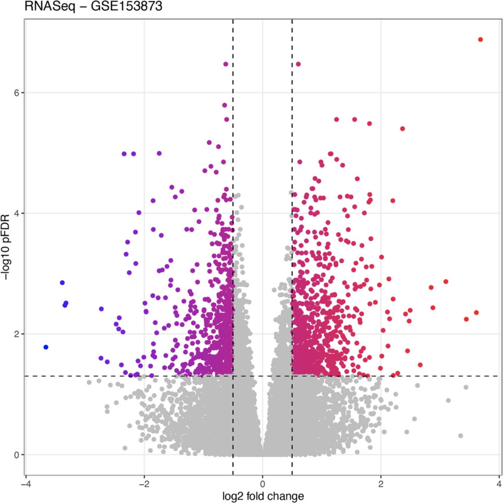
5.Visualize the differential analysis results using MA and volcano plots:
-
MA plot
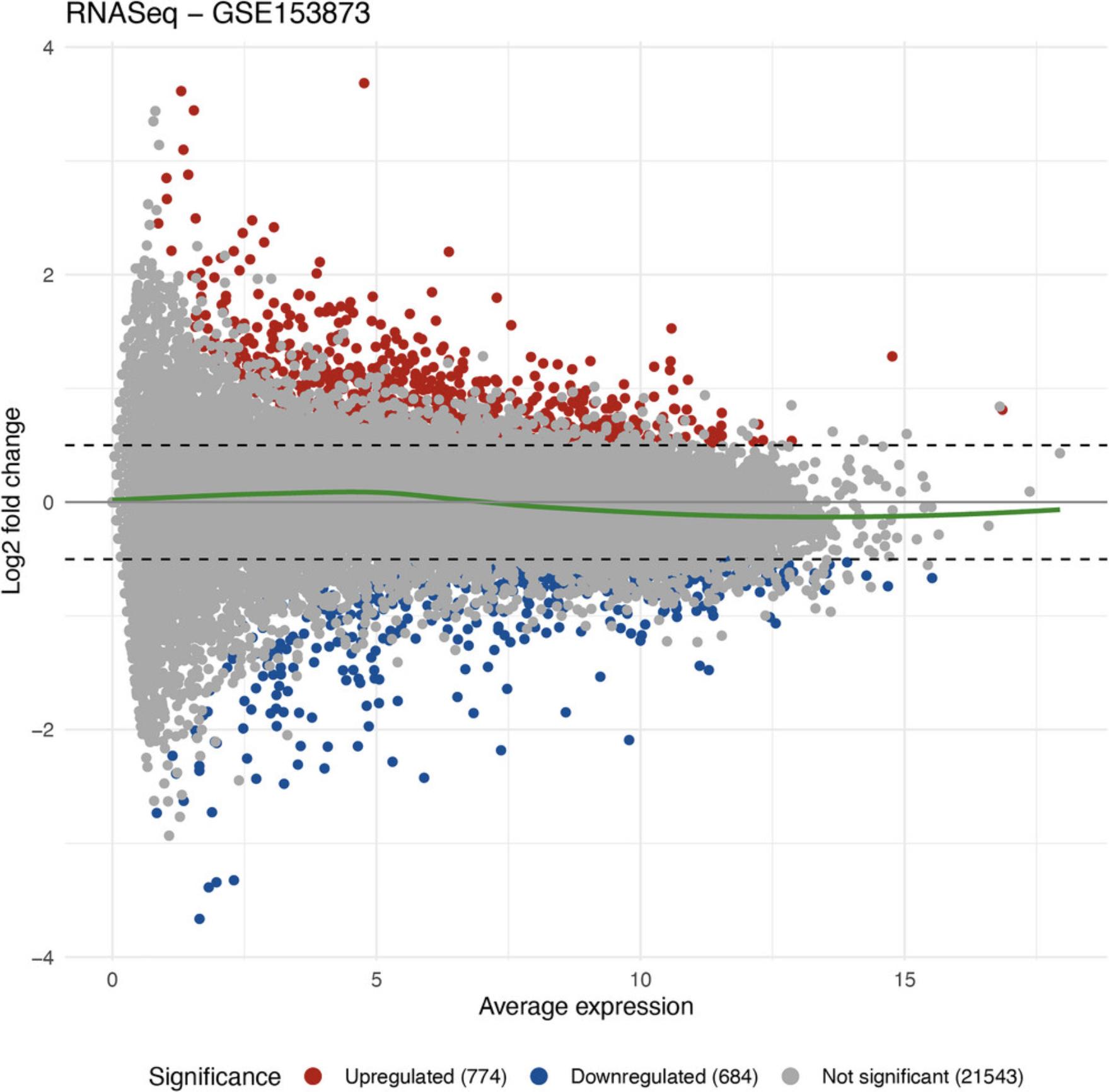
RCPA::plotMA(RNASeqDEResults, logFCThreshold = 0.5) +
ggplot2::ggtitle("RNASeq - GSE153873")
-
Volcano plot
RCPA::plotVolcanoDE(RNASeqDEResults, logFCThreshold = 0.5) +
ggplot2::ggtitle("RNASeq - GSE153873")
Basic Protocol 5: GENE SET ENRICHMENT ANALYSIS
Pathway analysis is a systems-level approach that translates differential expression evidence into meaningful biological insights. Within our RCPA package, we implement eight methods for pathway analysis, which can be classified into two groups: gene set enrichment analysis and topology-based (TB) analysis methods. Gene set enrichment analysis generally does not take pathway topology and gene interactions into account whereas topology-based (TB) pathway analysis methods consider pathway topology and gene interactions when performing pathway analysis (Nguyen et al., 2018).
This protocol provides step-by-step instructions for performing gene set enrichment analysis using the implemented function RCPA::runGeneSetAnalysis(). The methods implemented for enrichment analysis include the Kolmogorov-Smirnov (KS) test (Massey Jr, 1951), the Wilcoxon test (Wilcoxon, 1992), over-representation analysis (ORA) (Huang et al., 2009; Khatri et al., 2002), fast gene set enrichment analysis (FGSEA) (Korotkevich et al., 2021; Sergushichev, 2016), and gene set analysis (GSA) (Efron & Tibshirani, 2007).
Necessary Resources
Hardware
- An internet-connected computer or laptop with at least 8 GB of RAM and 20 GB of free hard drive space
Software
- R runtime environment (version 4.0.0 or later)
- RCPA package from the CRAN repository (see Internet Resources)
Besides the functions in RCPA, we will need to use the functions in the SummarizedExperiment package to access the data stored in the SummarizedExperiment object. Similarly, some functions from the ggplot2 package will be used to add the title or modify the figures generated by the plot functions in RCPA. We can ensure the required packages are installed by loading them as shown in the following code snippet:
- library(RCPA)
- library(SummarizedExperiment)
- library(ggplot2)
Files
- SummarizedExperiment object obtained from differential analysis outlined in Basic Protocols 3 and 4
- Sample files
Users can use the function RCPA::loadData() to load the pre-saved differential analysis results of the three datasets from our GitHub repository https://github.com/tinnlab/RCPA/tree/main/.data. The first step in this protocol will guide the user in loading the pre-saved data using the function.
1.If users skipped Basic Protocols 3 and 4, they could use the function RCPA::loadData() to load the results:
-
loading differential results for Affymetrix data
affyDEExperiment <- RCPA::loadData("affyDEExperiment")
-
loading the results for Agilent data
agilDEExperiment <- RCPA::loadData("agilDEExperiment")
-
loading the results for RNA-Seq data
RNASeqDEExperiment <- RCPA::loadData("RNASeqDEExperiment")
2.Download gene sets from KEGG or GO:
-
Download gene sets from KEGG for human
KEGGGenesets <- RCPA::getGeneSets(database = "KEGG", org = "hsa")
-
Display gene sets in R console
str(KEGGGenesets)
-
Console output
List of 3
$ database: chr "KEGG"
$ genesets:List of 355
..$ path:hsa00010: chr [1:67] "10327" "124" "125" "126" ...
..$ path:hsa00020: chr [1:30] "1431" "1737" "1738" "1743" ...
..$ path:hsa00030: chr [1:31] "132158" "2203" "221823" "226" ...
..$ path:hsa00040: chr [1:36] "10327" "10720" "10941" "231" ...
.. [list output truncated] ...
$ names : Named chr [1:340] "Glycolysis / Gluconeogenesis" "Citrate cycle (TCA cycle)" "Pentose phosphate pathway" "Pentose and glucuronate interconversions" ...
..- attr(*, "names")= chr [1:340] "path:hsa00010" "path:hsa00020" "path:hsa00030" "path:hsa00040" ...
-
Download the gene sets from GO database
GOTerms <- RCPA::getGeneSets(database = "GO", taxid = 9606, namespace = "biological_process")
-
Display GOTerms in R console
str(GOTerms)
-
Console output
List of 3
$ database: chr "GO"
$ genesets:List of 12386
..$ GO:0000002: chr [1:11] "291" "1890" "4205" "4358" ...
..$ GO:0000038: chr [1:19] "30" "51" "215" "225" ...
..$ GO:0000079: chr [1:49] "60" "595" "641" "890" ...
..$ GO:0000082: chr [1:66] "91" "586" "595" "596" ...
.. [list output truncated]
$ names : Named chr [1:12386] "mitochondrial genome maintenance" "very long-chain fatty acid metabolic process" "regulation of cyclin-dependent protein serine/threonine kinase activity" "G1/S transition of mitotic cell cycle" ...
..- attr(*, "names")= chr [1:12386] "GO:0000002" "GO:0000038" "GO:0000079" "GO:0000082" ...
3.Perform enrichment analysis using the Kolmogorov-Smirnov (KS) or Wilcoxon test:
-
Set seed to create reproducible results
set.seed(1)
-
Enrichment analysis using KS test and KEGG pathways
RNASeqKSResult <- RCPA::runGeneSetAnalysis(summarizedExperiment = RNASeqDEExperiment,genesets = KEGGGenesets, method = "ks")
-
Display the result for KS test
print(RNASeqKSResult[1:5, c("ID", "p.value", "pFDR", "score", "name")])
-
Console output
|
|
|
|
|
|
|
|
|
|
|
|
|
|
|
|
|
|
|
|
|
|
|
|
|
|
|
|
|
|
-
Enrichment analysis using Wilcoxon test and KEGG pathways
RNASeqWilcoxResult <- RCPA::runGeneSetAnalysis(summarizedExperiment = RNASeqDEExperiment, genesets = KEGGGenesets, method = "wilcox")
-
Display the result for Wilcoxon test
print(RNASeqWilcoxResult[1:5, c("ID", "p.value", "pFDR", "score", "name")])
Console output
|
|
|
|
|
|
|
|
|
|
|
|
|
|
|
|
|
|
|
|
|
|
|
|
|
|
|
|
|
|
4.Perform enrichment analysis using over-representation analysis (ORA):
-
Specify the threshold to identify DE genes, which are required for ORA
oraArgsList <- list(pThreshold = 0.05)
-
Set seed to create reproducible results
set.seed(1)
-
Enrichment analysis using ORA and KEGG pathways
RNASeqORAResult <- RCPA::runGeneSetAnalysis(summarizedExperiment = RNASeqDEExperiment,genesets = KEGGGenesets, method = "ora", ORAArgs = oraArgsList)
-
Display the result for ORA
print(RNASeqORAResult[1:5, c("ID", "p.value", "pFDR", "score", "name")])
-
Console output
|
|
|
|
|
|
|
|
|
|
|
|
|
|
|
|
|
|
|
|
|
|
|
|
|
|
|
|
|
|
5.Perform enrichment analysis using fast gene set enrichment analysis (FGSEA):
-
Specify a list of arguments tailored for FGSEA:
FGSEAArgsList <- list(minSize = 10)
-
Set seed to create reproducible results
set.seed(1)
-
Enrichment analysis using FSGEA and KEGG pathway
RNASeqFGSEAResult <- RCPA::runGeneSetAnalysis(summarizedExperiment = RNASeqDEExperiment,genesets = KEGGGenesets, method = "fgsea", FgseaArgs = FGSEAArgsList)
-
Display the result for FGSEA
print(RNASeqFGSEAResult[c(1:5), c("ID", "p.value", "pFDR", "score", "name")])
-
Console output
|
|
|
|
|
|
|
|
|
|
|
|
|
|
|
|
|
|
|
|
|
|
|
|
|
|
|
|
|
|
6.Perform enrichment analysis using gene set analysis (GSA):
-
Specify the list of arguments customized for GSA
GSAArgsList <- list(method = "maxmean", minsize = 15, maxsize = 500, nperms = 1000)
-
Set seed to create reproducible results
set.seed(1)
-
Enrichment analysis using GSA and KEGG pathways
RNASeqGSAResult <- RCPA::runGeneSetAnalysis(summarizedExperiment = RNASeqDEExperiment,genesets = KEGGGenesets, method = "gsa", GSAArgs = GSAArgsList)
-
Display the result for GSA
print(RNASeqGSAResult[c(1:5), c("ID", "p.value", "pFDR", "score", "name")])
-
Console output
|
|
|
|
|
|
|
|
|
|
|
|
|
|
|
|
|
|
|
|
|
|
|
|
|
|
|
|
|
|
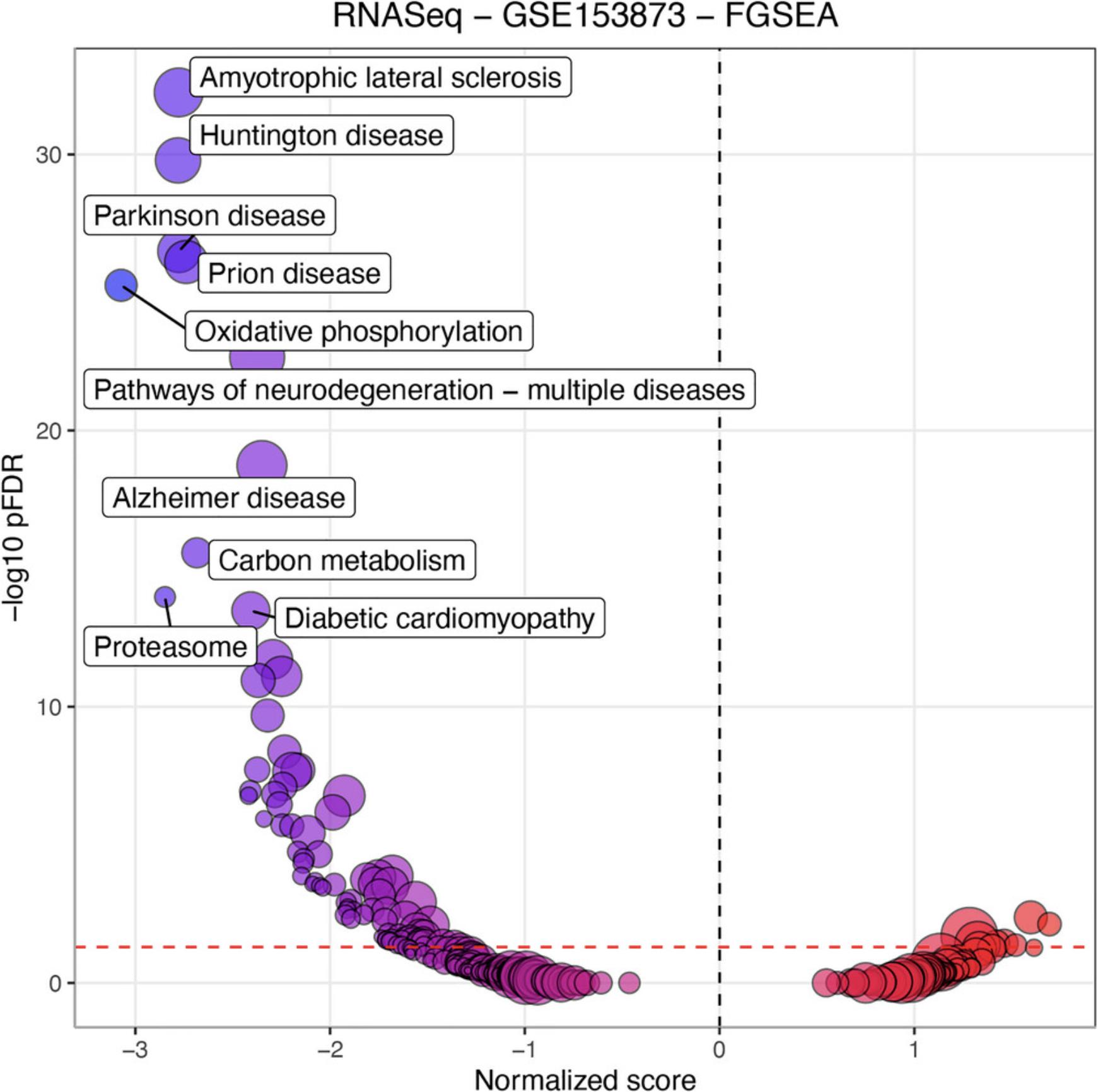
7.Visualize enrichment analysis results using volcano plot:
- RCPA::plotVolcanoPathway(PAResult = RNASeqFGSEAResult, topToLabel = 10) +
ggplot2::ggtitle("RNASeq - GSE153873 - FGSEA")
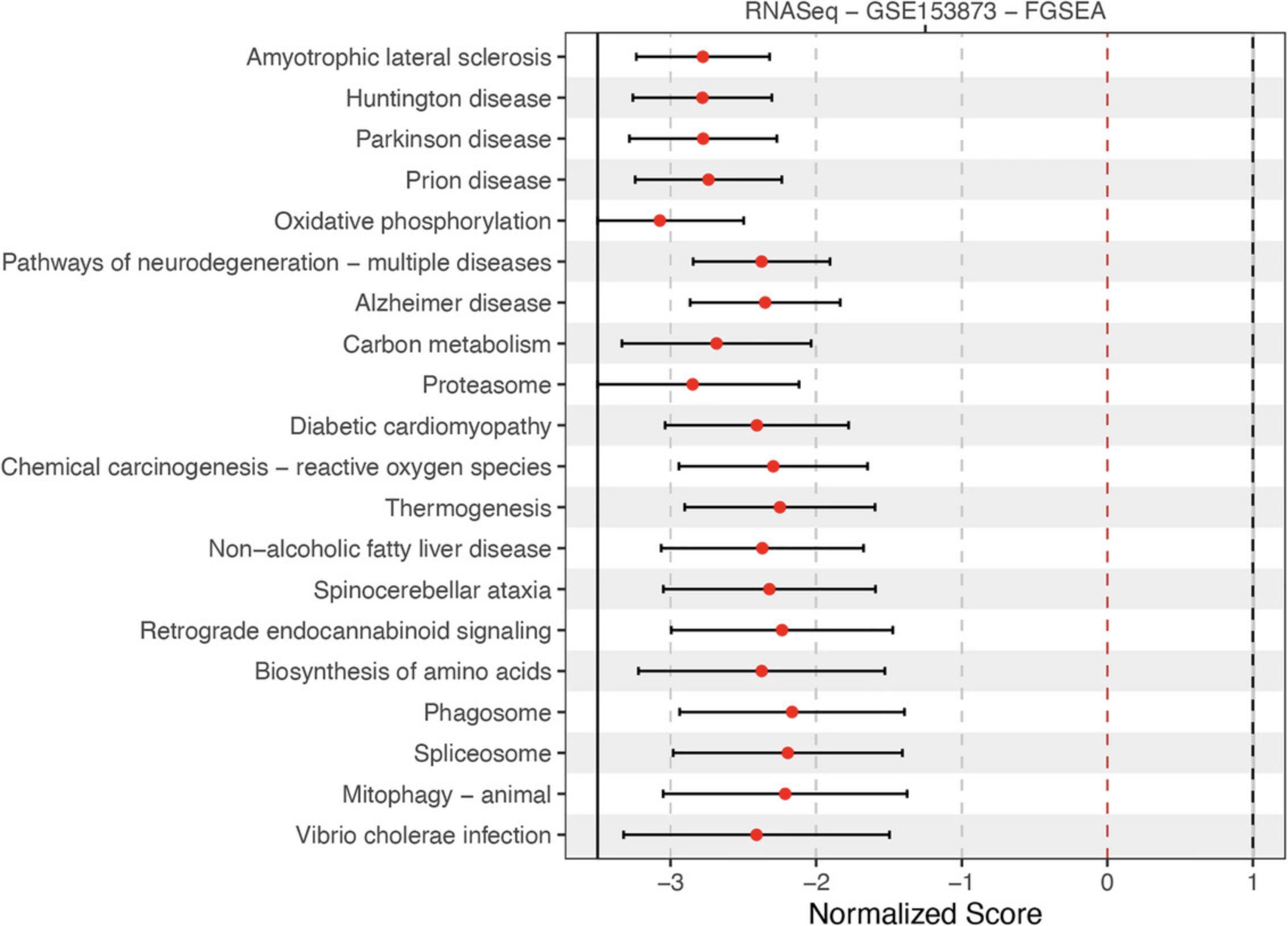
8.Visualize enrichment analysis results using forest plot:
-
Create a list containing top 20 pathways from the result
RNASeqFGSEAToPlot <- list("RNASeq - GSE153873 - FGSEA" = RNASeqFGSEAResult[1:20,])
-
Generate forest plot:
RCPA::plotForest(resultsList = RNASeqFGSEAToPlot, yAxis = "name", statLims = c(-3.5, 1))
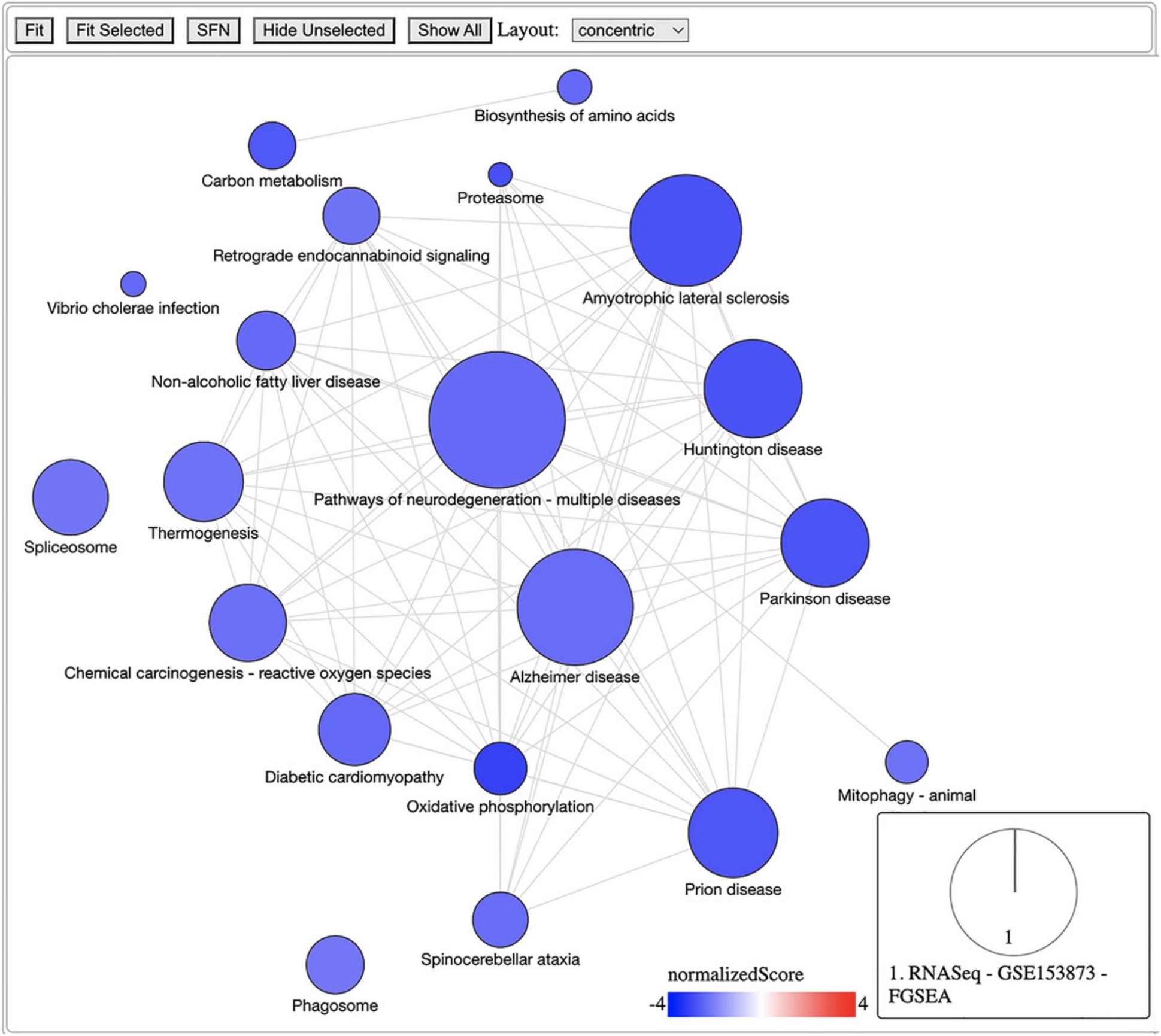
9.Visualize enrichment analysis results using a network graph of pathways:
-
Select the top 20 pathways from the results
RNASeqFGSEAToPlot <- list(“RNASeq -- GSE153873 -- FGSEA” = RNASeqFGSEAResult[1:20,])
-
Get IDs for top 20 pathways
selectedPathways <- RNASeqFGSEAResult$ID[1:20]
-
Generate network graph of selected pathways
pltHtml <- RCPA::plotPathwayNetwork(
PAResults = RNASeqFGSEAToPlot,
genesets = KEGGGenesets,
selectedPathways = selectedPathways,
statistic = “normalizedScore”,
mode = “continuous”,
edgeThreshold = 0.75,
file = tempfile(fileext = “.html”) # Or use a user-specified file path)
Basic Protocol 6: TOPOLOGY-BASED (TB) PATHWAY ANALYSIS
The previous protocol discusses gene set enrichment analysis using five different methods (Wilcoxon test, KS test, ORA, FGSEA, and GSA). Though powerful, enrichment methods do not take into consideration pathway topology and the interactions among the genes in the pathways. There exist also topology-based (TB) methods that consider pathway topology and gene interactions when performing pathway analysis. The RCPA package includes three TB methods: signaling pathway impact analysis (SPIA) (Draghici et al., 2007; Tarca et al., 2009), centrality-based pathway enrichment for ORA extension (CePa ORA), and for GSA extension (CePa GSA) (Gu et al., 2012; Gu & Wang, 2013). These methods are all accessible through the runPathwayAnalysis() function.
In addition to a SummarizedExperiment object that contains the differential analysis results, users need to provide pathways with gene interactions. In our context, each pathway is represented by a graph in which genes are nodes and edges are interactions among genes. Note that SPIA and CePa packages require completely different formats for their graph objects. To ease this process, we also include functions in RCPA that can automatically generate the required network data from KEGG for each method. These include getSPIAKEGGNetwork() for SPIA, and getCePaPathwayCatalogue() for CePa ORA and CePa GSA. If users want to understand more about the graph objects for these methods, they can consult the documentation for SPIA and CePa. Subsequently, users have the option to create their own network object, adhering to the same data structure used in SPIA and CePa, and supply it to the function runPathwayAnalysis().
Necessary Resources
Hardware
- An internet-connected computer or laptop with at least 8 GB of RAM and 20 GB of free hard drive space
Software
- R runtime environment (version 4.0.0 or later)
- RCPA package from the CRAN repository (see Internet Resources)
Besides the functions in RCPA, we will need to use the functions in the SummarizedExperiment to access the data stored in the SummarizedExperiment object. Similarly, some functions from the ggplot2 package will be used to add the title or modify the figures generated by the plot functions in RCPA. We can ensure the required packages are installed by loading them as shown in the following code snippet:
- library(RCPA)
- library(SummarizedExperiment)
- library(ggplot2)
Files
- SummarizedExperiment object obtained from differential analysis outlined in Basic Protocols 3 and 4
- Sample files
Users can use the function RCPA::loadData() to load the pre-saved differential analysis results of the three datasets from our GitHub repository (https://github.com/tinnlab/RCPA/tree/main/.data). The first step in this protocol will guide the user in loading the pre-saved data using the function.
1.If users skipped Basic Protocols 3 and 4, they can use RCPA::loadData() to load the results:
-
loading differential results for Affymetrix data
affyDEExperiment <- RCPA::loadData("affyDEExperiment")
-
loading the results for Agilent data
agilDEExperiment <- RCPA::loadData("agilDEExperiment")
-
loading the results for RNA-Seq data
RNASeqDEExperiment <- RCPA::loadData("RNASeqDEExperiment")
-
loading KEGG gene sets
KEGGGenesets <- RCPA::loadData("KEGGGenesets")
2.Retrieve pathway topology from KEGG for SPIA:
-
Retrieve gene networks from KEGG for SPIA
SPIANetwork <- RCPA::getSPIAKEGGNetwork(org = "hsa", updateCache = FALSE)
-
Display SPIANetwork
str(SPIANetwork)
-
Console output
List of 3
$ network:List of 312
.. $ path:hsa00010:Formal class 'graphNEL' [package "graph"] with 6 slots
.. ..@ nodes : chr [1:67] "226" "229" "230" "217" …
.. ..@ edgeL :List of 67
.. .. ..$ 226 :List of 1
.. .. .. ..$ edges: int [1:8] 45 46 42 43 44 41 39 40
.. .. ..$ 229 :List of 1
.. .. .. ..$ edges: int [1:8] 45 46 42 43 44 41 39 40
.. .. ..$ 230 :List of 1
.. .. .. ..$ edges: int [1:8] 45 46 42 43 44 41 39 40
.. .. ..$ 217 :List of 1
.. .. .. .. .. [list output truncated]
.. .. .. ..@ defaults:List of 1
.. .. .. .. ..$ subtype: logi NA
.. ..@ nodeData :Formal class 'attrData' [package "graph"] with 2 slots
.. .. .. ..@ data : Named list()
.. .. .. ..@ defaults: list()
.. ..@ renderInfo:Formal class 'renderInfo' [package "graph"] with 4 slots
.. .. .. ..@ nodes: list()
.. .. .. ..@ edges: list()
.. .. .. ..@ graph: list()
.. .. .. ..@ pars : list()
.. ..@ graphData :List of 1
.. .. ..$ edgemode: chr "directed"
.. [list output truncated] …
$ names: Named chr [1:312] "Glycolysis / Gluconeogenesis" "Citrate cycle (TCA cycle)" "Pentose phosphate pathway" "Pentose and glucuronate interconversions" …
..- attr(*, "names")= chr [1:312] "path:hsa00010" "path:hsa00020" "path:hsa00030" "path:hsa00040" …
$ sizes: Named int [1:312] 67 30 31 36 34 32 30 36 49 47 …
..- attr(*, "names")= chr [1:312] "path:hsa00010" "path:hsa00020" "path:hsa00030" "path:hsa00040" …
3.Perform topology-based (TB) pathway analysis using SPIA:
-
Specify the list of arguments specific for SPIA
SPIAArgsList <- list(nB = 1000, pThreshold = 0.05)
-
Set seed to create reproducible results
set.seed(1)
-
Run SPIA on RNA-Seq dataset
RNASeqSPIAResult <- RCPA::runPathwayAnalysis(summarizedExperiment = RNASeqDEExperiment,network = SPIANetwork, method = "spia", SPIAArgs = SPIAArgsList)
-
Display the result for dataset
print(RNASeqSPIAResult[1:5, c("ID", "p.value", "pFDR", "score", "name")])
-
Console output
|
|
|
|
|
|
|
|
|
|
|
|
|
|
|
|
|
|
|
|
|
|
|
|
|
|
|
|
|
|
4.Retrieve pathway topology from KEGG for CePa ORA and CePa GSA:
-
Retrieve pathway information from KEGG for CePa ORA and CePa GSA:
CePaNetwork <- RCPA::getCePaPathwayCatalogue(org = "hsa", updateCache = FALSE)
-
Display CePaNetwork
str(CePaNetwork)
-
Console output
List of 3
$ network:List of 3
..$ pathList :List of 312
.. ..$ path:hsa00010: chr [1:268] "1" "2" "3" "4" …
.. ..$ path:hsa00020: chr [1:101] "269" "270" "271" "272" …
.. ..$ path:hsa00030: chr [1:158] "1" "2" "3" "4" …
.. ..$ path:hsa00040: chr [1:75] "508" "509" "510" "511" …
.. .. [list output truncated]
..$ interactionList:'data.frame': 62995 obs. of 3 variables:
.. ..$ interaction.id: chr [1:62995] "1" "2" "3" "4" …
.. ..$ input : chr [1:62995] "226" "226" "226" "226" …
.. ..$ output : chr [1:62995] "2203" "8789" "5211" "5213" …
..$ Mapping :'data.frame': 7758 obs. of 2 variables:
.. ..$ node.id: chr [1:7758] "226" "229" "230" "217" …
.. ..$ symbol : chr [1:7758] "226" "229" "230" "217" …
..- attr(*, "class")= chr "pathway.catalogue"
$ names: Named chr [1:312] "Glycolysis / Gluconeogenesis" "Citrate cycle (TCA cycle)" "Pentose phosphate pathway" "Pentose and glucuronate interconversions" …
..- attr(*, "names")= chr [1:312] "path:hsa00010" "path:hsa00020" "path:hsa00030" "path:hsa00040" …
$ sizes: Named int [1:312] 268 101 158 75 138 74 101 192 154 223 …
..- attr(*, "names")= chr [1:312] "path:hsa00010" "path:hsa00020" "path:hsa00030" "path:hsa00040" …
5.Perform pathway analysis using CePa ORA:
-
Specify the list of argument tailored for CePa ORA
CePaORAArgsList <- list(cen = "equal.weight", pThreshold = 0.05)
-
Set seed to create reproducible results
set.seed(1)
-
Run CePa ORA
RNASeqCePaORAResult <- RCPA::runPathwayAnalysis(summarizedExperiment = RNASeqDEExperiment,network = CePaNetwork, method = "cepaORA", CePaORAArgs = CePaORAArgsList)
-
Display the result
print(RNASeqCePaORAResult[1:5, c("ID", "p.value", "pFDR", "score", "name")])
-
Console output
|
|
|
|
|
|
|
|
|
|
|
|
|
|
|
|
|
|
|
|
|
|
|
|
|
|
|
|
|
|
6.Perform pathway analysis using CePa GSA:
-
Specify the list of argument tailored for CePa GSA
CePaGSAArgsList <- list(cen = "equal.weight", nlevel = "tvalue_abs", plevel = "mean")
-
Set seed to reproducible results
set.seed(1)
-
Run CePa GSA on RNA-Seq dataset
RNASeqCePaGSAResult <- RCPA::runPathwayAnalysis(summarizedExperiment = RNASeqDEExperiment,network = CePaNetwork, method = "cepaGSA", CePaGSAArgs = CePaGSAArgsList)
-
Display the result
print(RNASeqCePaGSAResult[1:5, c("ID", "p.value", "pFDR", "score", "name")])
-
Console output
|
|
|
|
|
|
|
|
|
|
|
|
|
|
|
|
|
|
|
|
|
|
|
|
|
|
|
|
|
|
7.Visualize pathway analysis results using volcano, forest plot, and network of pathways:
-
Generate volcano plot for SPIA results
RCPA::plotVolcanoPathway(PAResult = RNASeqSPIAResult, topToLabel = 15) +
ggplot2::ggtitle("RNASeq - GSE153873 - SPIA")
Figure 17 shows the volcano plot for the results obtained from SPIA. Similar to the visualization for gene set enrichment analysis, users can easily visualize the volcano plot for TB pathway analysis using the function plotVolcanoPathway().
-
Select the top 20 pathways from the results
RNASeqSPIAToPlot <- list("RNASeq - GSE153873 - SPIA" = RNASeqSPIAResult[1:20,])
selectedPathways <- RNASeqSPIAResult$ID[1:20]
-
Generate forest plot:
RCPA::plotForest(resultsList = RNASeqSPIAToPlot, yAxis = "name", statLims = c(-4, 8))
Using the code snippet above, users can visualize the forest plot, as shown in Figure 18. The figure shows the pathway score and their confidence interval for the 20 most significant pathways obtained from SPIA analysis.
-
Generate network graph of selected pathways
pltHtml <- RCPA::plotPathwayNetwork(
PAResults = RNASeqSPIAToPlot,
genesets = KEGGGenesets,
selectedPathways = selectedPathways,
statistic = "normalizedScore",
mode = "continuous",
edgeThreshold = 0.75)
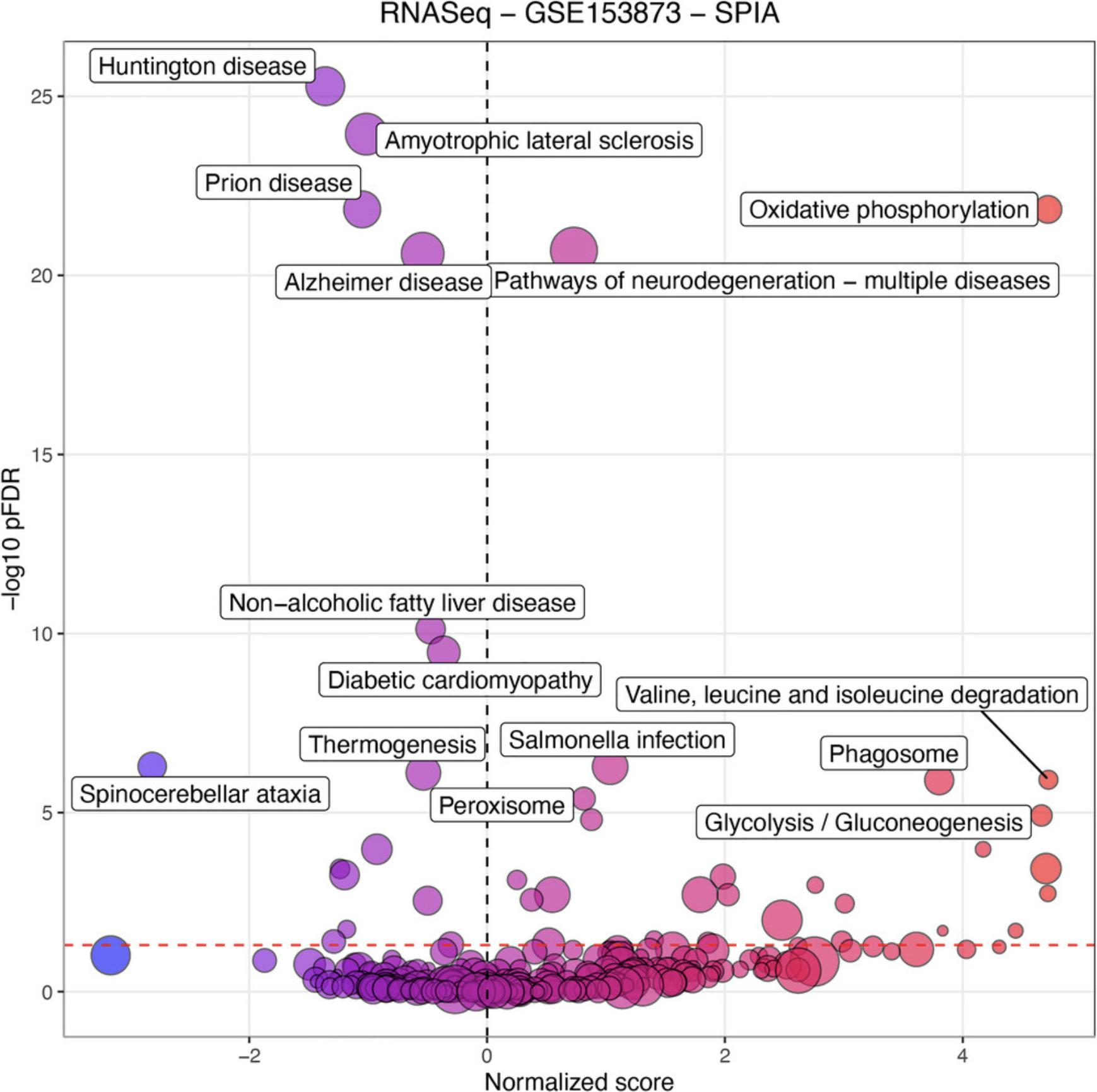
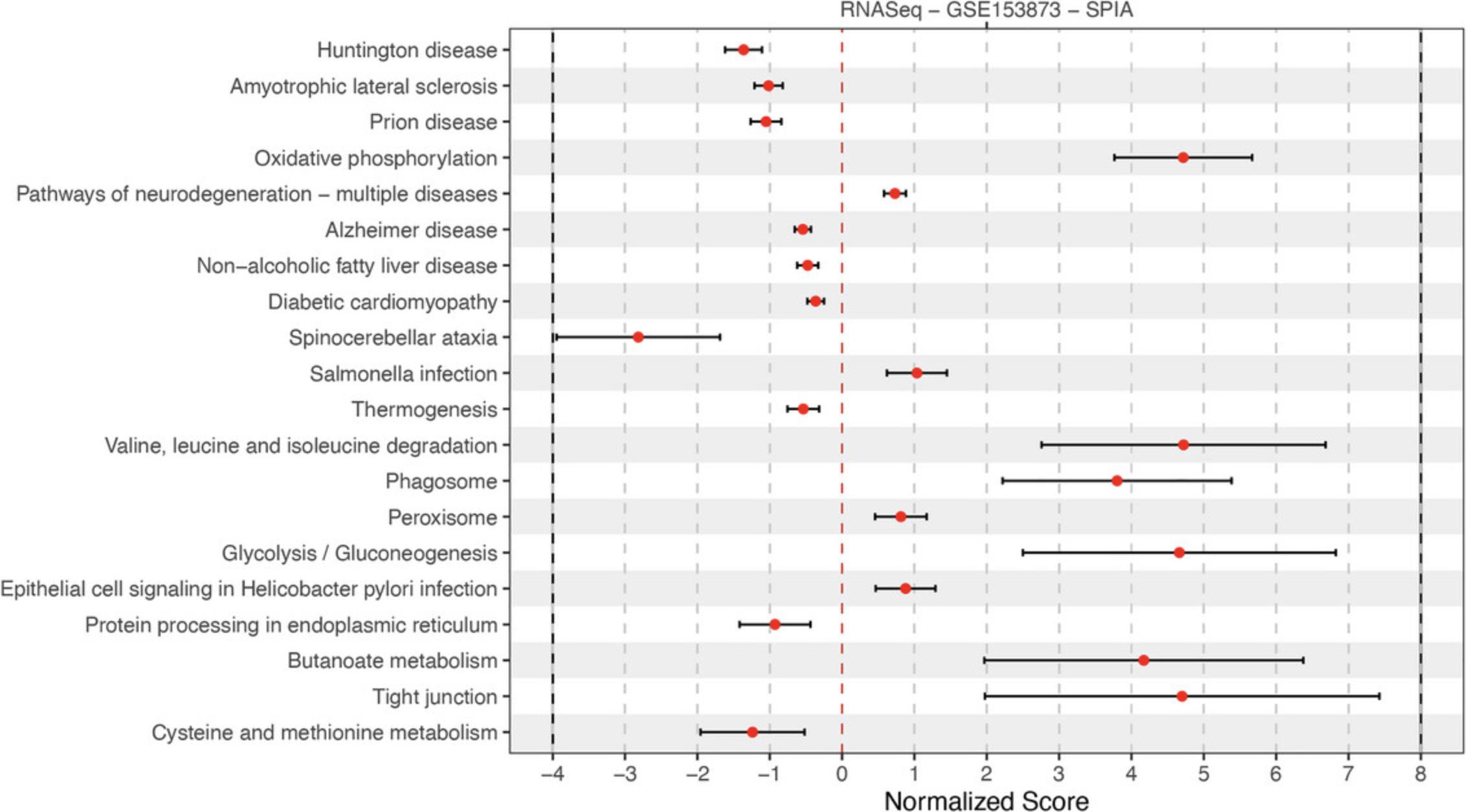
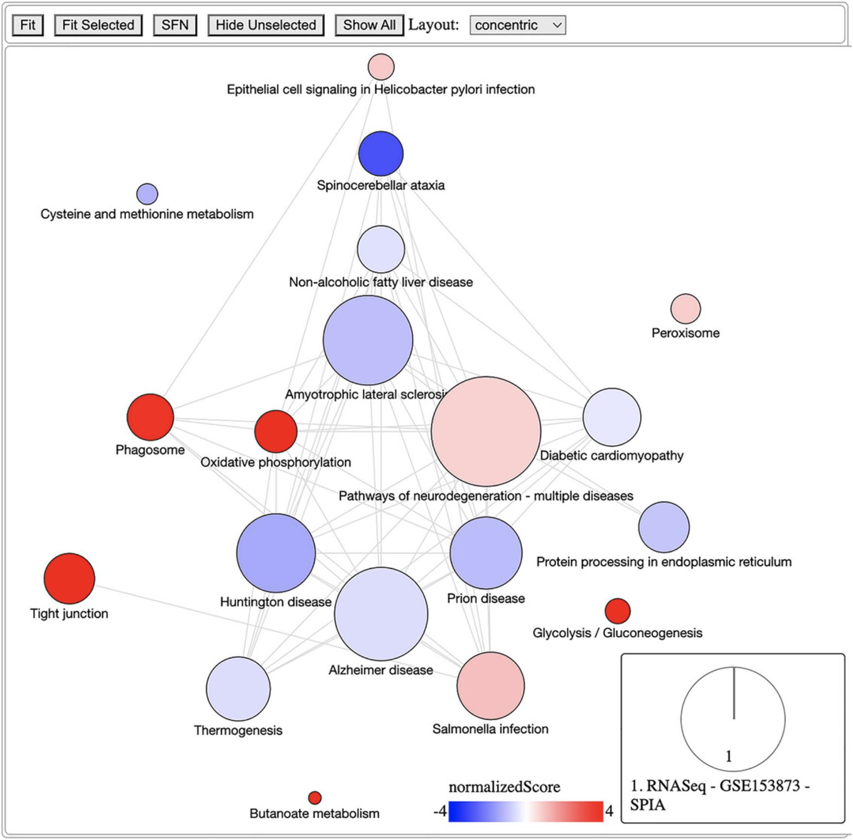
Basic Protocol 7: DATA INTEGRATION AND VISUALIZATION
This protocol describes the RCPA functions that are of integrating and visualizing analysis results obtained from multiple datasets and analysis methods. We introduce two distinct kinds of integrative analysis strategies: meta-analysis and consensus analysis. Meta-analysis is a set of statistical approaches used to combine multiple independent but related studies (Normand, 1999). Meta-analysis can potentially increase the statistical power of analysis methods and improve the accuracy of the findings. In contrast, consensus analysis involves merging the outcomes derived from different analyses, resulting in a unified and consolidated conclusion, as shown in our previous publication (Nguyen et al., 2021). This strategy allows users to compare the results of multiple methods. Using consensus pathway analysis, users can observe the effects of the underlying hypotheses that form the basis of the analysis methods of interest. Consensus pathway analysis can be extended to include results obtained from multiple datasets and methods at the same time to understand the effects of method hypothesis, experiment design, and other factors.
Using the RCPA package, meta-analysis can be performed at both gene- and pathway-level, while consensus analysis is only performed at the pathway-level. In the following example, we still use the same three GEO datasets, GSE5281 (Affymetrix), GSE61196 (Agilent), and GSE153873 (RNA-Seq). Note that all three datasets study the same condition: Alzheimer's disease.
Necessary Resources
Hardware
- An internet-connected computer or laptop with at least 8 GB of RAM and 20 GB of free hard drive space
Software
- R runtime environment (version 4.0.0 or later)
- RCPA package from the CRAN repository (see Internet Resources)
Besides the functions in RCPA, we will need to use the functions in the SummarizedExperiment to access the data stored in the SummarizedExperiment object. Similarly, some functions from the ggplot2 package will be used to add the title or modify the figures generated by the plot functions in RCPA. We can ensure the required packages are installed by loading them as shown in the following code snippet:
- library(RCPA)
- library(SummarizedExperiment)
- library(ggplot2)
Files
- SummarizedExperiment objects obtained from differential analysis outlined in Basic Protocols 3 and 4
- Data frame containing gene set enrichment and/or pathway analysis results described in Basic Protocols 5 and 6, to perform pathway-level meta-analysis and consensus analysis
- Sample files
Users can use the function RCPA::loadData() to load the pre-saved data and analysis results of the three datasets in the previous protocols from our GitHub repository (https://github.com/tinnlab/RCPA/tree/main/.data). There are detailed steps in this protocol that guide the users in loading the pre-saved data using the function.
Gene-level meta-analysis
Here we illustrate how users can combine the differential analysis results obtained from multiple datasets. We assume that users have performed differential analysis and pathway analysis using our previous protocols, and that these results are stored in SummarizedExperiment objects, namely affyDEExperiment, agilDEExperiment, and RNASeqDEExperiment, as described in Basic Protocols 3 and 4.
1.If users skipped Basic Protocols 3 and 4, they can use the function RCPA::loadData() to load the results:
-
DE analysis result from Affymetrix dataset:
affyDEExperiment <- RCPA::loadData("affyDEExperiment")
-
DE analysis result from Agilent dataset:
agilDEExperiment <- RCPA::loadData("agilDEExperiment")
-
DE analysis result from RNA-Seq dataset:
RNASeqDEExperiment <- RCPA::loadData("RNASeqDEExperiment")
2.Compile differential expression results of multiple datasets into a list:
-
Extract the differential analysis result obtained from previous protocols
affyDEResults <- SummarizedExperiment::rowData(affyDEExperiment)
agilDEResults <- SummarizedExperiment::rowData(agilDEExperiment)
RNASeqDEResults <- SummarizedExperiment::rowData(RNASeqDEExperiment)
-
Prepare the input list of DE results
DEResults <- list(
"Affymetrix - GSE5281" = affyDEResults,
"Agilent - GSE61196" = agilDEResults,
"RNASeq - GSE153873" = RNASeqDEResults)
3.Generate a Venn diagram and query common genes:
-
Generate a venn diagram plot
RCPA::plotVennDE(DEResults = DEResults, topToList = 10)
-
Retrieve a list of common DE genes among multiple datasets
commonDEGenes <- RCPA::getCommonDEGenes(DEResults = DEResults)
-
Display the results
print(commonDEGenes[1:5,])
-
Console output:
|
|
|
|
|
|
|
|
|
|
|
|
|
|
|
|
|
|
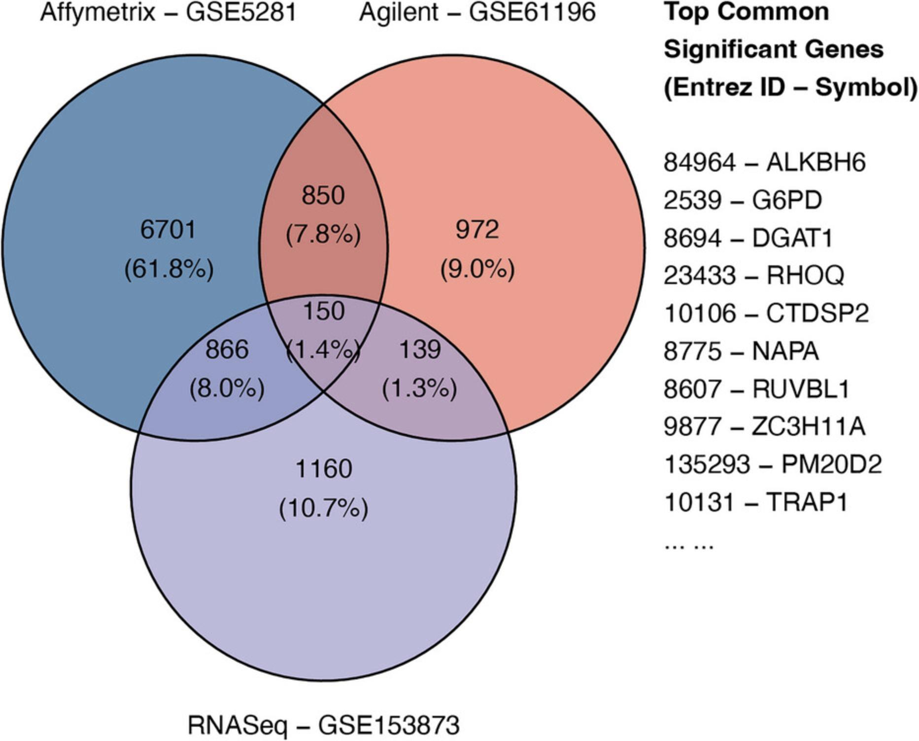
4.Perform meta-analysis using one of the six methods:
-
Perform meta-analysis using Stouffer's method
metaDEResult <- RCPA::runDEMetaAnalysis(DEResults = DEResults, method = "stouffer")
-
Display the result:
head(metaDEResult)
-
Console output
|
|
|
|
|
|
|
|
|
|
|
|
|
|
|
|
|
|
|
|
|
|
|
|
|
|
|
|
|
|
|
|
|
|
|
5.Visualize meta-analysis results using gene heatmap:
-
Select the top 40 most significant genes:
genesToPlot <- metaDEResult$ID[1:40]
-
Get the full description of the genesToPlot:
genesAnnotation <- RCPA::getEntrezAnnotation(genesToPlot)
labels <- genesAnnotation[genesToPlot, "Description"]
-
Create a list containing the results from individual analysis and meta analysis
affyDEResults <- SummarizedExperiment::rowData(affyDEExperiment)
agilDEResults <- SummarizedExperiment::rowData(agilDEExperiment)
RNASeqDEResults <- SummarizedExperiment::rowData(RNASeqDEExperiment)
resultsToPlot <- list(
"Affymetrix - GSE5281" = affyDEResults,
"Agilent - GSE61196" = agilDEResults,
"RNASeq - GSE153873" = RNASeqDEResults,
"Meta-analysis" = metaDEResult)
-
Generate gene heatmap
RCPA::plotDEGeneHeatmap(DEResults = resultsToPlot, genes = genesToPlot, labels = labels,negLog10pValueLims = c(0, 5), logFCLims = c(-1, 1))
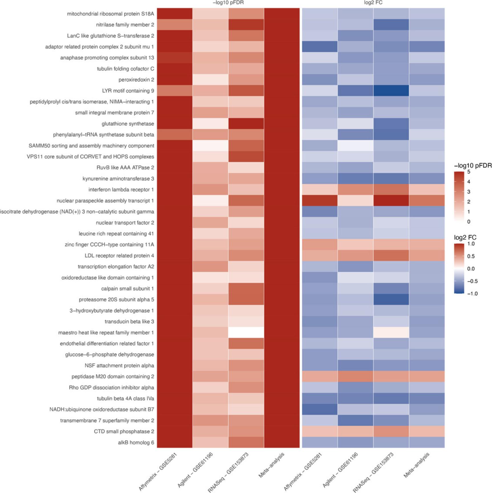
6.Visualize a KEGG pathway with gene statistics:
-
Select columns in the results of differential analysis:
selectedColumns <- colnames(metaDEResult)
print(selectedColumns)
Console output
[1] "ID" "p.value" "pFDR" "logFC" "logFCSE"
-
Prepare the list for plotting
DEResultsToPlot <- list(
"Affymetrix - GSE5281" = affyDEResults[, selectedColumns],
"Agilent - GSE61196" = agilDEResults[, selectedColumns],
"RNASeq - GSE153873" = RNASeqDEResults[, selectedColumns],
"Meta-analysis" = metaDEResult)
-
Plot for KEGG Alzheimer's Disease pathway
pltObj <- RCPA::plotKEGGMap(DEResults = DEResultsToPlot, KEGGPathwayID = "hsa05010", stat = "logFC", pThreshold = 1, statLimit = 1)
-
Display the plot
pltObj$plot
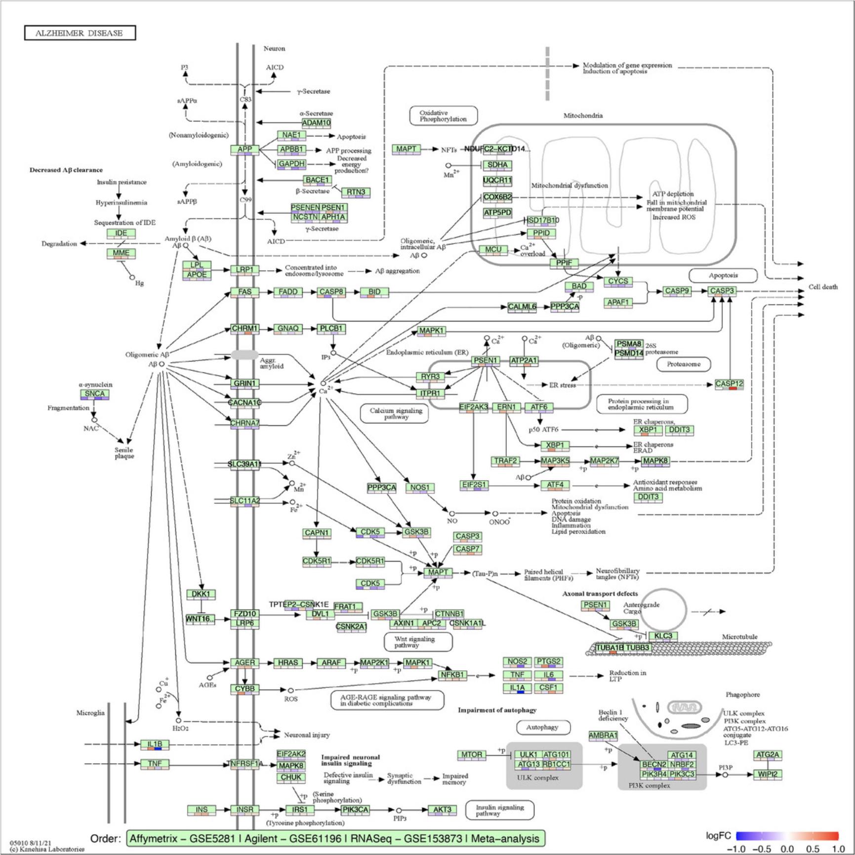
Pathway-level meta-analysis
Here we illustrate how users can combine pathway analysis results obtained from multiple datasets. We assume that users have performance gene set enrichment analysis or pathway analysis, as described in Basic Protocols 5 and 6.In the following, we will combine the results obtained from FGSEA across the three datasets GSE5281, GSE61196, and GSE153873.
7.If users skipped Basic Protocols 5 and 6, they could use the function RCPA::loadData() to load the enrichment results obtained from the method FGSEA for all three datasets:
-
FGSEA analysis result from Affymetrix dataset:
affyFGSEAResult <- RCPA::loadData("affyFGSEAResult")
-
FGSEA analysis result from Agilent dataset:
agilFGSEAResult <- RCPA::loadData("agilFGSEAResult")
-
FGSEA analysis result from RNA-Seq dataset:
RNASeqFGSEAResult <- RCPA::loadData("RNASeqFGSEAResult")
-
Load the KEGG gene sets
KEGGGenesets <- RCPA::loadData("KEGGGenesets")
8.Prepare a list of pathway analysis results from multiple datasets:
-
Compile a list of pathway analysis results
PAResults <- list(
"Affymetrix - GSE5281" = affyFGSEAResult,
"Agilent - GSE61196" = agilFGSEAResult,
"RNASeq - GSE153873" = RNASeqFGSEAResult)
9.Generate a Venn diagram and query common pathways:
-
Plot venn diagram
RCPA::plotVennPathway(PAResults = PAResults, pThreshold = 0.05)
-
Query a list of common pathways
commonPathways <- RCPA::getCommonPathways(PAResults = PAResults)
-
Display the results:
print(commonPathways[1:5,])
-
Console output:
|
|
|
|
|
|
|
|
|
|
|
|
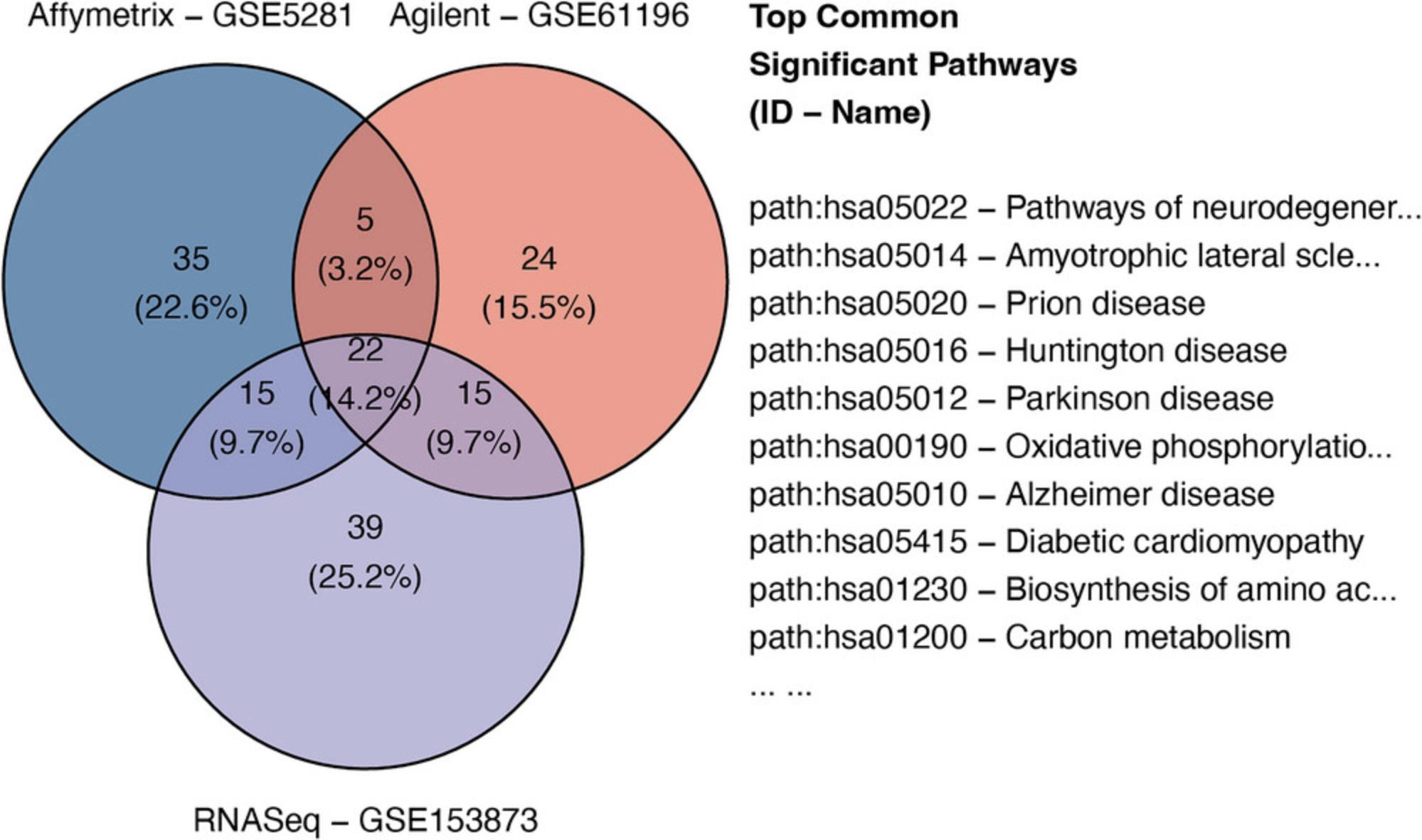
10.Perform pathway-level meta-analysis using one of the six methods:
-
Meta-analysis using Stouffer's method
metaPAResult <- RCPA::runPathwayMetaAnalysis(PAResults = PAResults, method = "stouffer")
-
Display the results:
print(metaPAResult[1:5, 1:5])
-
Console output
|
|
|
|
|
|
|
|
|
|
|
|
|
|
|
|
|
|
|
|
|
|
|
|
|
|
|
|
|
|
11.Generate a bar chart for pathway-level meta-analysis:
-
Select the top 30 significant from meta-analysis
selectedPathways <- metaPAResult$ID[1:30]
-
Create a list of pathway analysis results of these 30 pathways
PAResultsToPlot <- list(
"Affymetrix - GSE5281" = affyFGSEAResult,
"Agilent - GSE61196" = agilFGSEAResult,
"RNASeq - GSE153873" = RNASeqFGSEAResult,
"Meta-analysis" = metaPAResult)
-
Plot bar chart
RCPA::plotBarChart(results = PAResultsToPlot, selectedPathways = selectedPathways) +ggplot2::ggtitle("FGSEA Analysis Results")
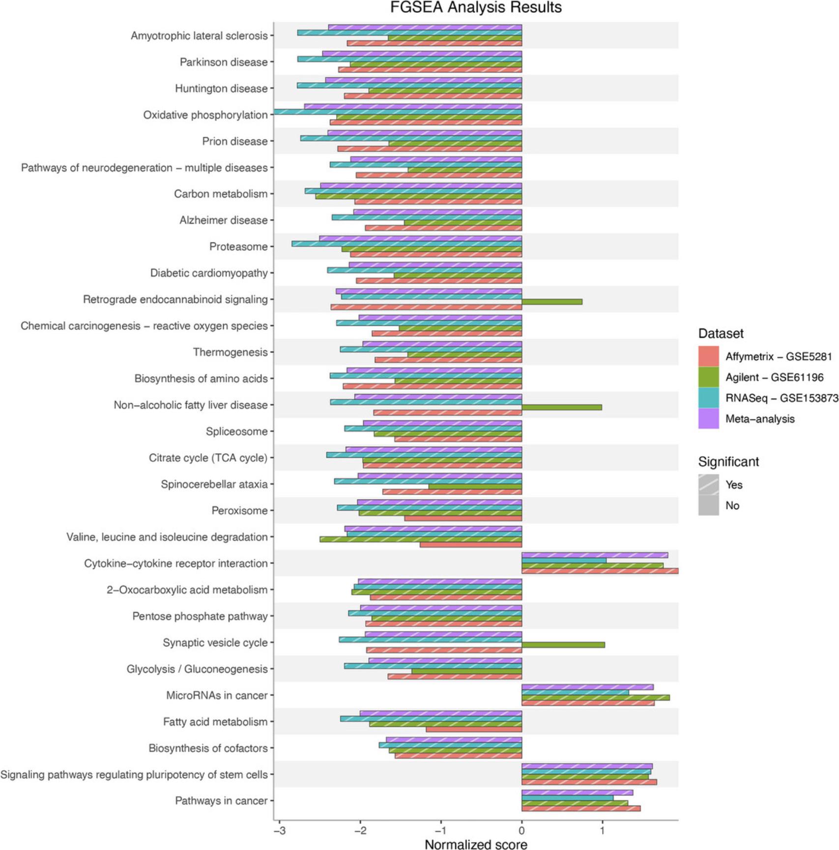
12.Generate a pathway heatmap for meta-analysis:
- RCPA::plotPathwayHeatmap(resultsList = PAResultsToPlot, yAxis = "name", selectedPathways = selectedPathways)
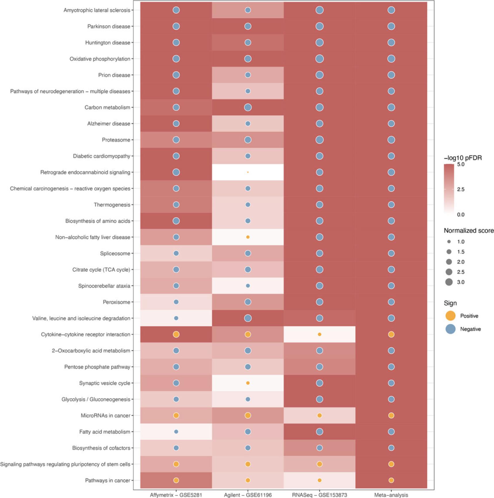
13.Generate a pathway network for meta-analysis:
-
Select the top 30 significant from meta-analysis
selectedPathways <- metaPAResult$ID[1:30]
-
Create a list of pathway analysis results of these 30 pathways
allPAResultsToPlot <- list(
"Affymetrix - GSE5281" = affyFGSEAResult,
"Agilent - GSE61196" = agilFGSEAResult,
"RNASeq - GSE153873" = RNASeqFGSEAResult,
"Meta-analysis" = metaPAResult)
-
Plot pathway network
pltHtml <- RCPA::plotPathwayNetwork(
PAResults = allPAResultsToPlot,
genesets = KEGGGenesets,
selectedPathways = selectedPathways,
statistic = "normalizedScore",
mode = "continuous",
edgeThreshold = 0.75)
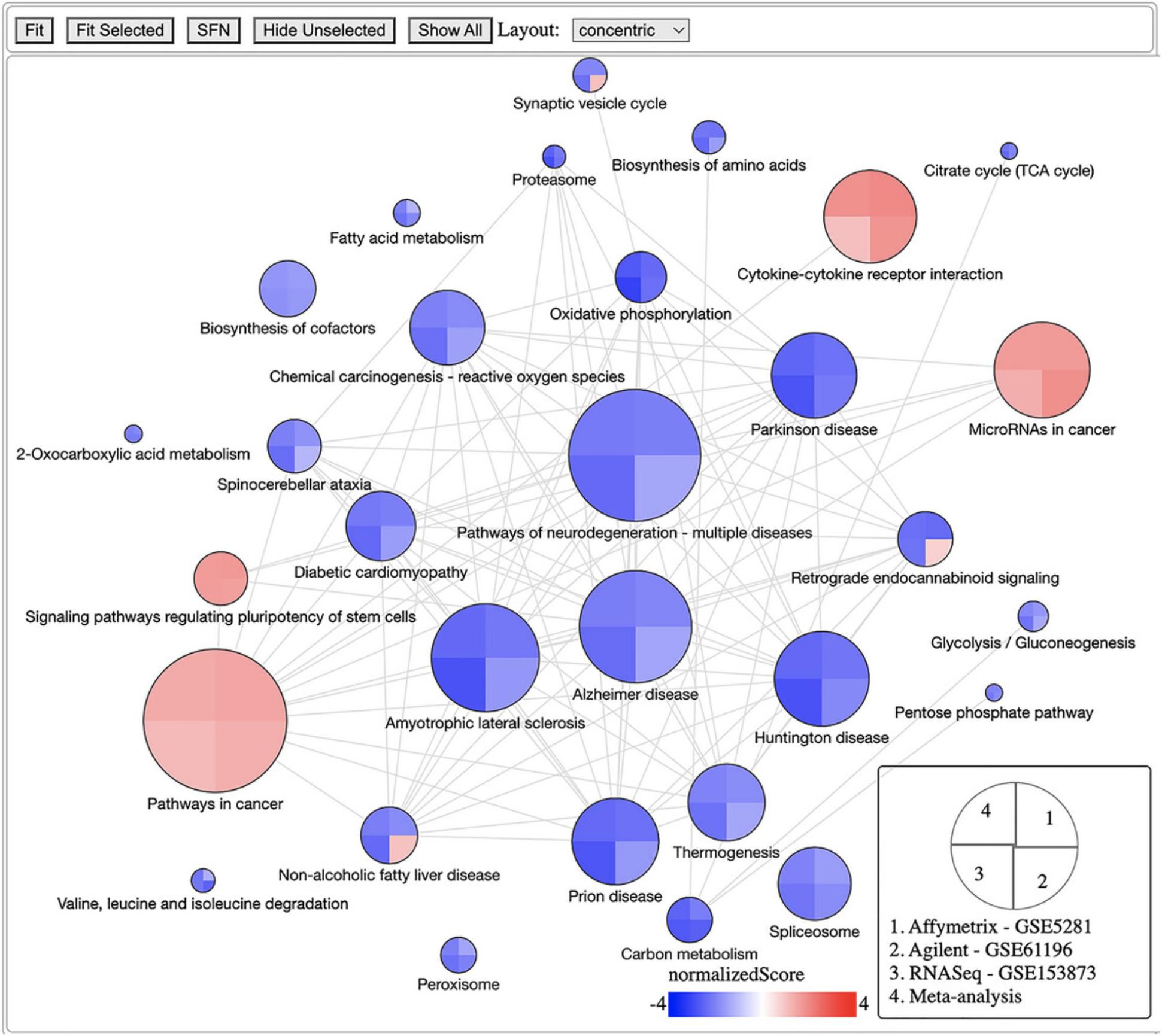
Pathway-level consensus analysis
The main objective of consensus pathway analysis is to allow users to see the differences, as well as the consensus results across many methods that rely on distinctively different hypotheses. As a result, it helps life scientists who are trying to understand the underlying biological mechanisms of a condition or disease of interest. Consensus analysis can also be extended to compare multiple experiments and computational methods so that users can compare different hypotheses, experimental designs, and technologies. Below we illustrate the application of consensus pathway analysis to combine the pathway analysis results obtained from three methods and three datasets.
14.If users skipped the previous protocols for pathway analysis, they could use RCPA::loadData() to load the data:
-
Wilcoxon test results for RNA-Seq dataset:
RNASeqWilcoxResult <- RCPA::loadData("RNASeqWilcoxResult")
-
FGSEA results for RNA-Seq dataset:
RNASeqFGSEAResult <- RCPA::loadData("RNASeqFGSEAResult")
-
SPIA results for RNA-Seq dataset:
RNASeqSPIAResult <- RCPA::loadData("RNASeqSPIAResult")
-
Load the KEGG gene sets
KEGGGenesets <- RCPA::loadData("KEGGGenesets")
15.Prepare the input list of analysis results for consensus analysis:
-
Prepare a list of results obtained from the Wilcox test, FGSEA, and SPIA
selectedRNASeqPAResults <- list(
"Wilcox" = RNASeqWilcoxResult,
"FGSEA" = RNASeqFGSEAResult,
"SPIA" = RNASeqSPIAResult)
16.Generate a Venn diagram for the three analyses:
-
Plot Venn diagram
RCPA::plotVennPathway(PAResults = selectedRNASeqPAResults, pThreshold = 0.05)
-
Query a list of common pathways from Wilcox Test, FGSEA, SPIA:
commonPathways <- RCPA::getCommonPathways(PAResults = selectedRNASeqPAResults)
-
Display the result
print(commonPathways[1:5,])
-
Console output
|
|
|
|
|
|
|
|
|
|
|
|
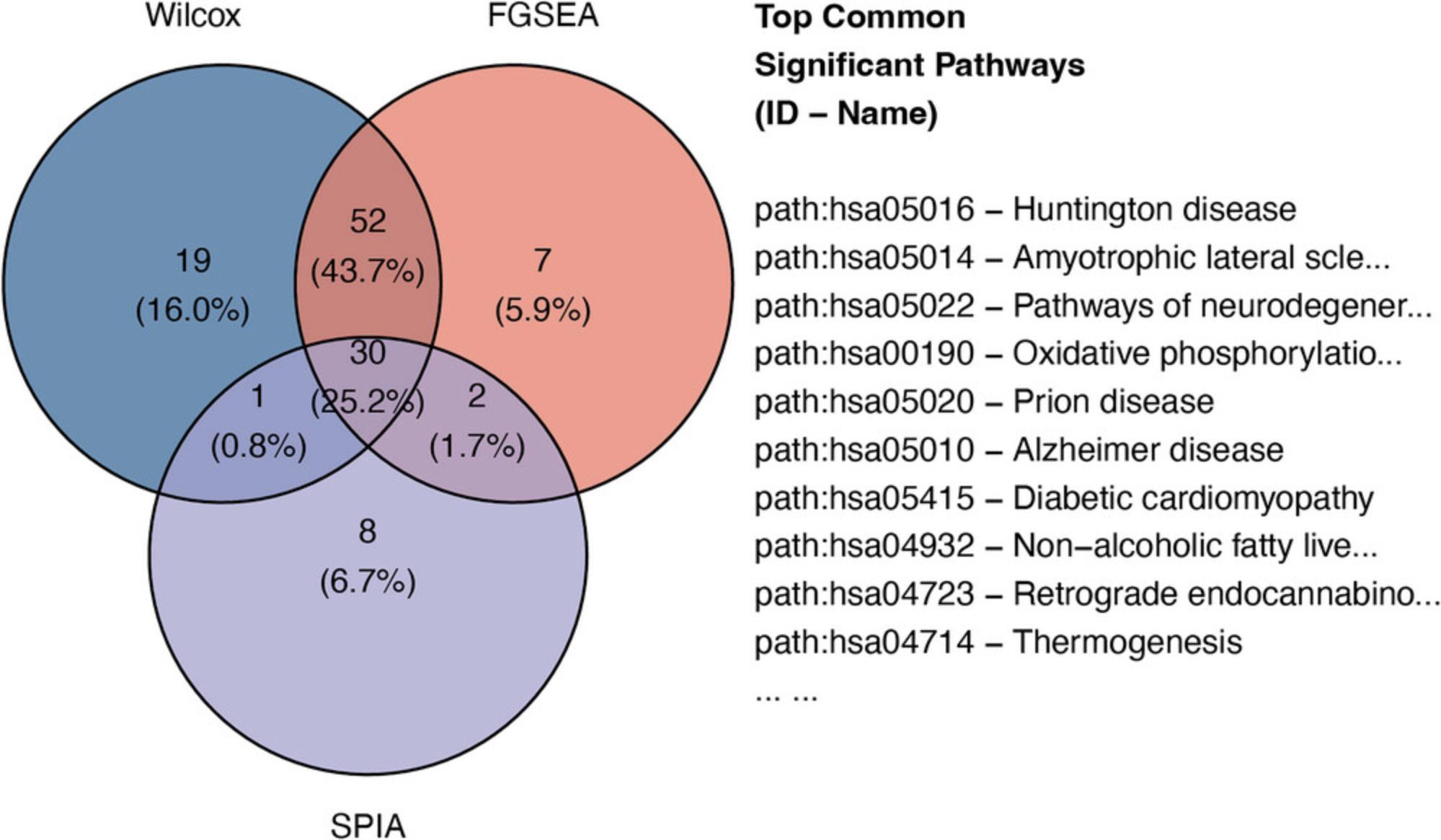
17.Perform consensus analysis using the weightedZMean method:
-
Set seed to create reproducible result:
set.seed(1)
-
Run consensus analysis
consensusWZRNASeqPAResult <- RCPA::runConsensusAnalysis(PAResults = selectedRNASeqPAResults, method = "weightedZMean")
-
Display the result
print(consensusWZRNASeqPAResult[1:6, c("ID", "p.value", "pFDR", "name")])
-
Console output
|
|
|
|
|
|
|
|
|
|
|
|
|
|
|
|
|
|
|
|
|
|
|
|
|
|
|
|
18.Perform consensus analysis using robust rank aggregation:
-
Set seed to create reproducible result:
set.seed(1)
-
Run consensus analysis
consensusRRARNASeqPAResult <- RCPA::runConsensusAnalysis(PAResults = selectedRNASeqPAResults, method = "RRA", rank.by = "both")
-
Display the result
print(consensusRRARNASeqPAResult[1:5, c("ID", "p.value", "pFDR", "name")])
-
Console output
|
|
|
|
|
|
|
|
|
|
|
|
|
|
|
|
|
|
|
|
|
|
|
|
19.Generate pathway network for consensus analysis:
-
Create a list of results to plot:
selectedCCRNASeqPAResults <- list(
"Wilcox" = RNASeqWilcoxResult,
"FGSEA" = RNASeqFGSEAResult,
"SPIA" = RNASeqSPIAResult,
"Consensus - weightedZMean" = consensusWZRNASeqPAResult
)
-
Select to plot top 30 most significant pathways
from consensus analysis using weightedZMean:
selectedPathways <- consensusWZRNASeqPAResult$ID[1:30]
-
Plot pathway network
pltHtml <- RCPA::plotPathwayNetwork(
PAResults = selectedCCRNASeqPAResults,
genesets = KEGGGenesets,
selectedPathways = selectedPathways,
statistic = "p.value",
mode = "discrete",
pThreshold = 0.05,
edgeThreshold = 0.75)
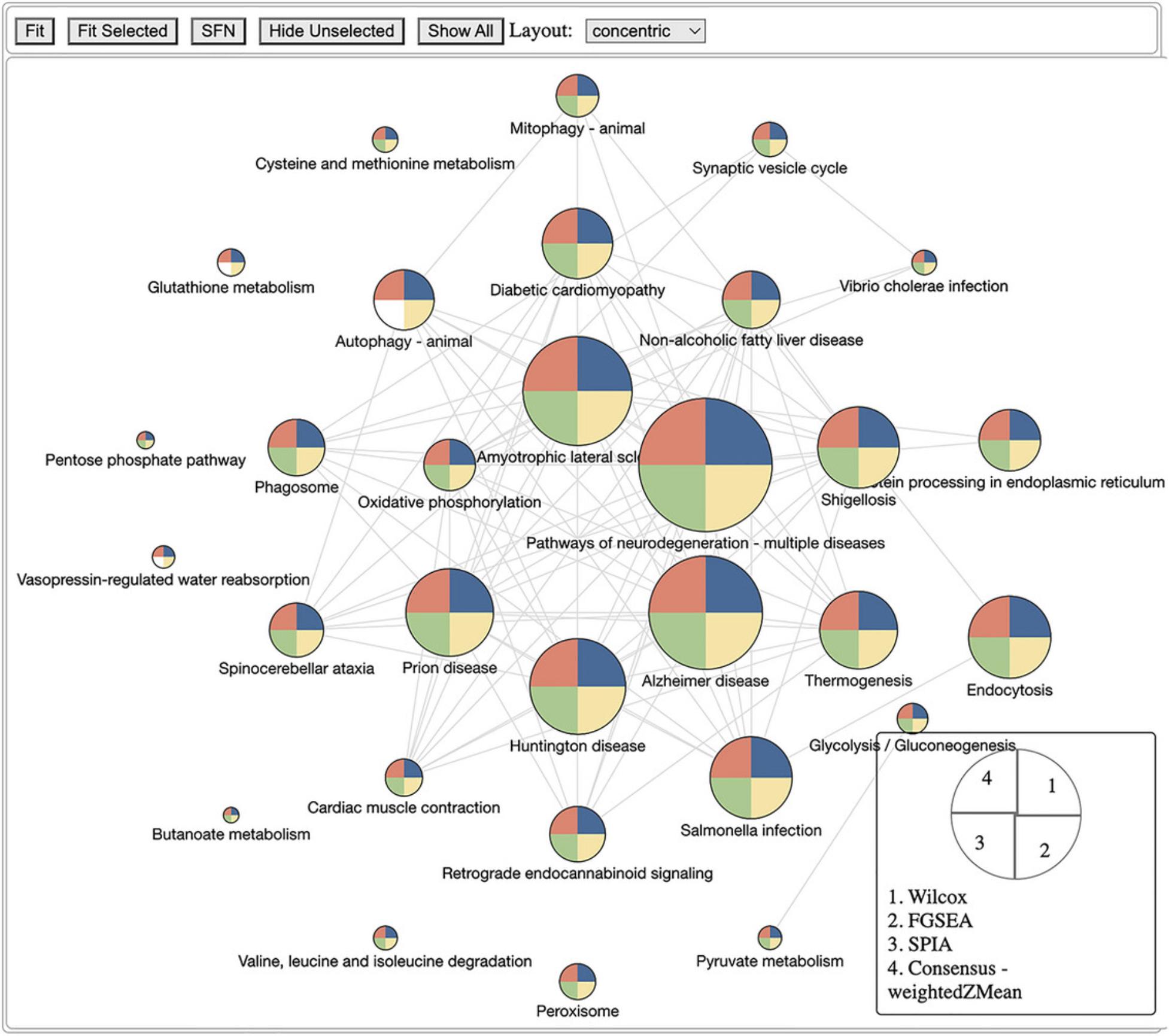
20.Perform consensus analysis of multiple methods and datasets:
-
Load the necessary data if users skipped the previous protocols
Enrichment results using Wilcoxon test:
affyWilcoxResult <- RCPA::loadData("affyWilcoxResult")
RNASeqWilcoxResult <- RCPA::loadData("RNASeqWilcoxResult")
agilWilcoxResult <- RCPA::loadData("agilWilcoxResult")
-
Enrichment results FGSEA:
affyFGSEAResult <- RCPA::loadData("affyFGSEAResult")
agilFGSEAResult <- RCPA::loadData("agilFGSEAResult")
RNASeqFGSEAResult <- RCPA::loadData("RNASeqFGSEAResult")
-
TB analysis using SPIA:
affySPIAResult <- RCPA::loadData("affySPIAResult")
agilSPIAResult <- RCPA::loadData("agilSPIAResult")
RNASeqSPIAResult <- RCPA::loadData("RNASeqSPIAResult")
-
Load the KEGG gene sets
KEGGGenesets <- RCPA::loadData("KEGGGenesets")
-
Create a list of results from multiple pathway analysis methods and datasets:
selectedPAResults <- list(
"Affymetrix - Wilcox" = affyWilcoxResult,
"Affymetrix - FGSEA" = affyFGSEAResult,
"Affymetrix - SPIA" = affySPIAResult,
"Agilent - Wilcox" = agilWilcoxResult,
"Agilent - FGSEA" = agilFGSEAResult,
"Agilent - SPIA" = agilSPIAResult,
"RNASeq - Wilcox" = RNASeqWilcoxResult,
"RNASeq - FGSEA" = RNASeqFGSEAResult,
"RNASeq - SPIA" = RNASeqSPIAResult)
-
Run consensus analysis using weightedZMean on selectedPAResults:
consensusPAResult <- RCPA::runConsensusAnalysis(PAResults = selectedPAResults, method = "weightedZMean")
-
display the results
print(consensusPAResult[1:6, c("ID", "p.value", "pFDR", "name")])
-
Console output:
|
|
|
|
|
|
|
|
|
|
|
|
|
|
|
|
|
|
|
|
|
|
|
|
|
|
|
|
-
Select the top 20 significant from consensus analysis
selectedPathways <- consensusPAResult$ID[1:20]
-
Create a list of results to plot:
selectedPAResultsToPlot <- list(
"Affymetrix - Wilcox" = affyWilcoxResult,
"Affymetrix - FGSEA" = affyFGSEAResult,
"Affymetrix - SPIA" = affySPIAResult,
"Agilent - Wilcox" = agilWilcoxResult,
"Agilent - FGSEA" = agilFGSEAResult,
"Agilent - SPIA" = agilSPIAResult,
"RNASeq - Wilcox" = RNASeqWilcoxResult,
"RNASeq - FGSEA" = RNASeqFGSEAResult,
"RNASeq - SPIA" = RNASeqSPIAResult,
"Consensus Analaysis" = consensusPAResult)
-
Plot pathway network
pltHtml <- RCPA::plotPathwayNetwork(
PAResults = selectedPAResultsToPlot,
genesets = KEGGGenesets,
selectedPathways = selectedPathways,
statistic = "p.value",
mode = "discrete",
edgeThreshold = 0.75)
Figure 29 shows the pathway network graph obtained from the above code. Users can perform consensus analysis on many different pathway analysis results, which can be obtained from different methods and/or different datasets, by following the same procedure as shown in the above code. Here, we performed gene set and pathway analysis using three methods: Wilcox test, FGSEA and SPIA on three GEO datasets. In return, we obtained 9 different pathway analysis results in total. We then perform consensus analysis on these results using weightedZMean. Next, we also use the plotPathwayNetwork() to generate the pathway network for consensus pathway analysis results. The figure shows the top 20 most significant pathways from consensus analysis.
- RCPA::plotPathwayHeatmap(resultsList = selectedPAResultsToPlot, yAxis = "name",selectedPathways = selectedPathways)
Figure 30 shows the pathway heatmap obtained from the function plotPathwayHeatmap() to plot the pathway heatmap for the 9 pathway analysis results and their consensus analysis. The function requires the following inputs: (1) resultsList, a named list of data frames from pathway analysis; (2) yAxis, a character parameter specifying which column of the result data frame from pathway analysis is used to label to y-axis; and (3) selectedPathways, the IDs of pathways to be shown in the plot (NULL by default). The plotPathwayHeatmap() also returns a ggplot object as other plot functions that have been introduced thus far. Note that since each analysis method has its own distinct definition of an enrichment score, we do not combine the scores across the methods in consensus analysis.
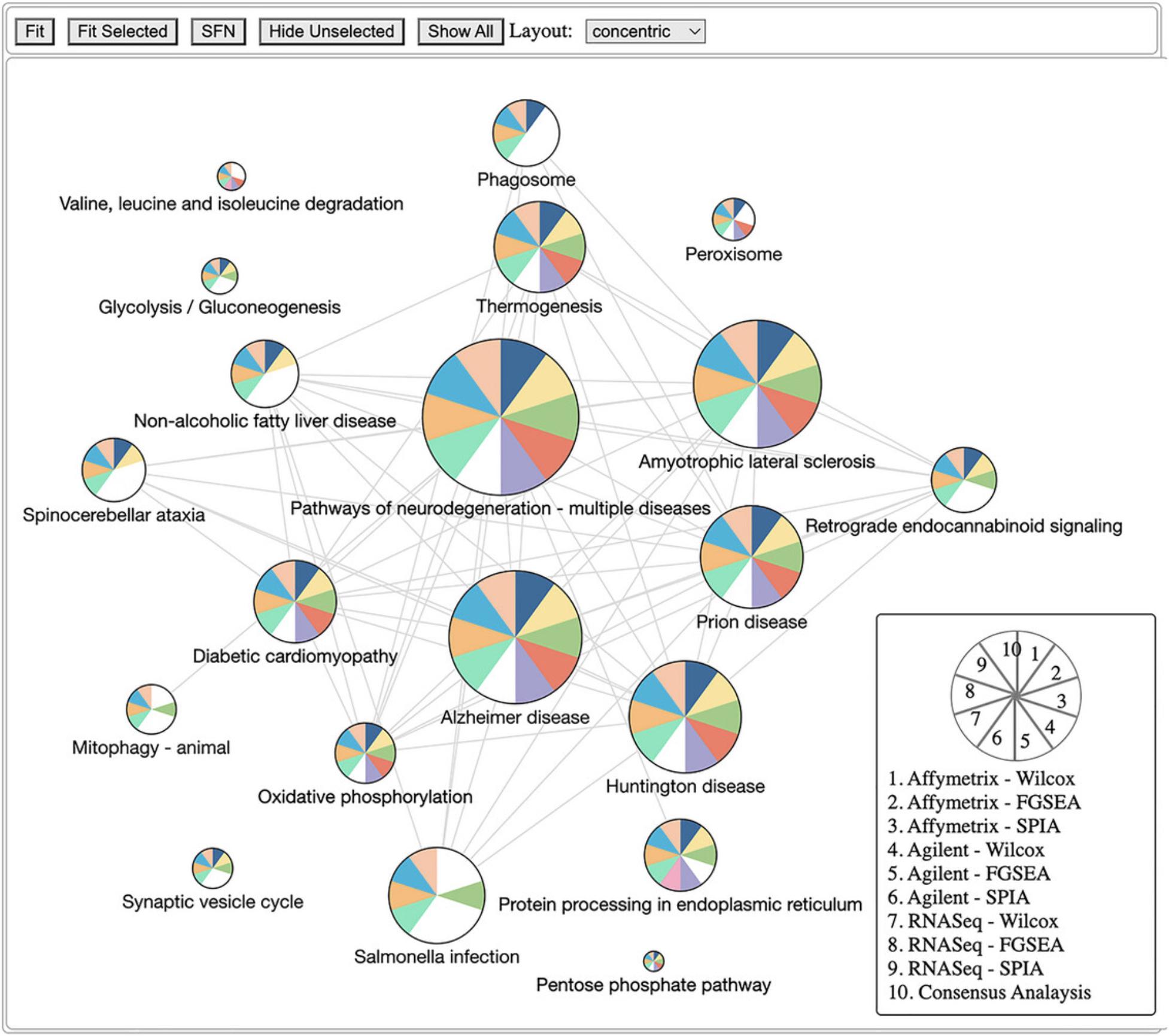
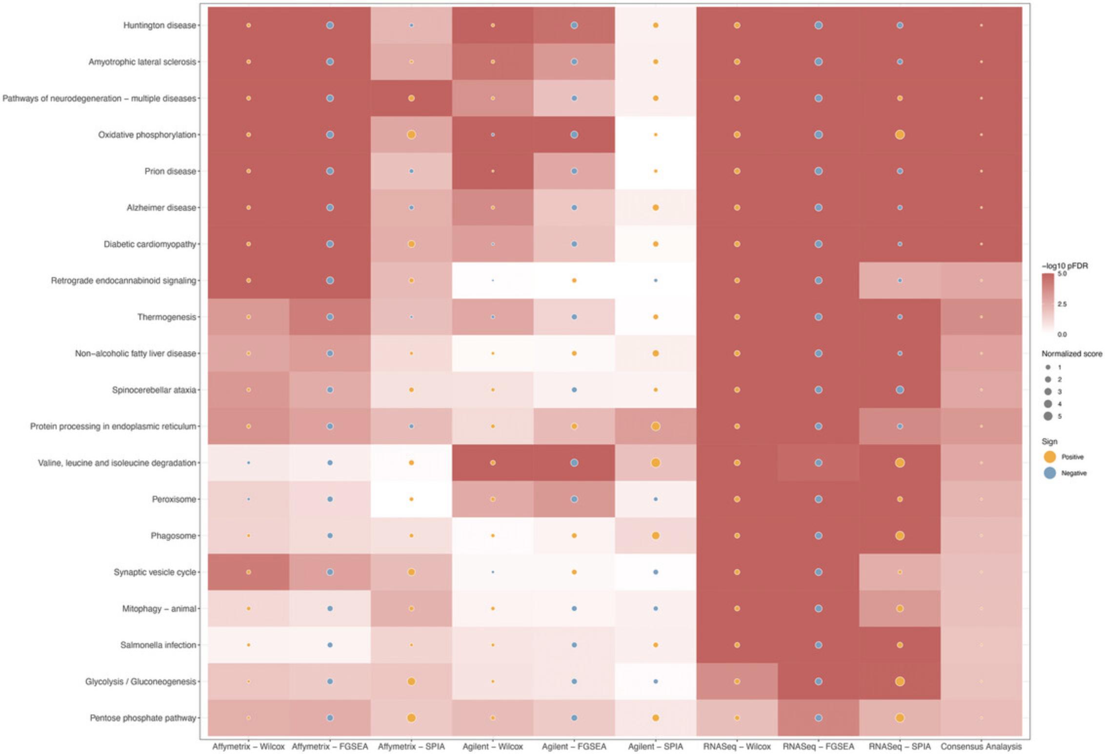
COMMENTARY
Background Information
In this article, we present a comprehensive and user-friendly pipeline implemented in the RCPA package for the complete analysis of gene expression data using various statistical and computational methods. The package includes many functions that allow users to perform: (1) data processing for microarray and RNA-Seq data NCBI GEO; (2) differential analysis using limma, edgeR, and DESeq2; (3) gene set enrichment analysis using the KS test, Wilcox test, ORA, FGSEA, and GSA; (4) topology-based pathway analysis using SPIA, CePa ORA, and CePa GSA; (5) meta-analysis using Fisher's method, Stouffer's method, geometric mean, minP, addCLT, and REML; (6) consensus analysis using weightedZMean and RRA methods; and (7) visualization of analysis results.
We illustrate the applications of those functions on several public datasets, showing its ability to identify differentially expressed genes, significant gene sets, impacted pathways, and consensus results obtained from meta-analysis and consensus analysis. The implemented functions also offer the flexibility to adjust the analysis parameters, making them useful for researchers with diverse experimental designs and objectives. While our package provides a comprehensive solution for gene expression analysis, we acknowledge that there is always room for improvement and extension. Future directions for our work could include incorporating additional methods and pathway databases for pathway analysis to enhance the pipeline's accuracy and efficiency.
In conclusion, we believe that our package will be a valuable resource for life scientists and practitioners. We hope that the package will facilitate the discovery of new insights into the molecular mechanisms underlying biological processes and diseases. We plan to continue improving and updating our package in response to emerging challenges and opportunities in molecular data analysis.
Critical Parameters
Users need to ensure that the experimental design is appropriate and accounts for any confounding variables, such as age, gender, or treatment duration, etc. The design matrix used in the analysis should accurately reflect the study design and avoid any linear dependencies. Furthermore, they should choose appropriate statistical thresholds to identify differentially expressed genes and/or enriched/impacted pathways/gene sets, such as adjusted p -values or false discovery rate (FDR) cutoffs. These thresholds should balance the tradeoff between sensitivity and specificity.
Troubleshooting
Table 2 provides a list of common problems that users may encounter when using our pipeline, along with possible solutions. For other potential problems, users can contact the maintainer of the package at https://cran.r-project.org/package=RCPA (see Internet Resources).
| Problem | Possible cause | Solution |
|---|---|---|
| Error when installing RCPA | Missing dependencies | RCPA includes some other R packages as dependencies; it is likely that system libraries are missing causing some R packages to fail to install; users need to carefully check the error shown in their console and try to install the missing libraries |
|
downloadGEO() function returns empty data frame |
No supplementary files are available | Some GEO datasets do not have supplementary files uploaded; in this case, users need to check the dataset on NCBI GEO to see if the supplementary files are available; if not, users can manually download the preprocessed data and create the SummarizedExperiment object. |
| makeContrasts() function returns name error | Special characters in column names | The makeContrasts() function in the limma package requires the column names to be valid R variable names; in this case, users can remove special characters from the column names and try again |
|
Large fold-change and statistic in the output of limma |
The input data is not log-transformed | The limma package requires log-transformed data as input |
| GSA returns large scores | The input data is not log-transformed | GSA requires log-transformed data as input |
| CePa cannot find samples for analysis | The contrast matrix has >2 conditions | CePa only supports comparative analysis between two conditions; the contrast matrix should only contain two columns, e.g., “normal” and “disease” |
| The text in the plots is too small | The default font size is too small for the plot size | Plots are generated using the ggplot2 package; the plot object can be freely modified using functions from the ggplot2 package |
| The saved plots are different from the plots shown in the R | The graphics device is not set properly | Users can apply the function ggplot2::ggsave() to save the plots instead of using the save button from their IDE |
Acknowledgments
This work was partially supported by the NSF (grant no. 2343019 and 2203236), NASA (grant no. 80NSSC22M0255, subaward 23-42), NIH NIGMS (grant no. 1R44GM152152-01), and NIH NCI (grant no. 1U01CA274573-01A1). Any opinions, findings, and conclusions or recommendations expressed in this material are those of the authors and do not necessarily reflect the views of any of the funding agencies.
Author Contributions
Hung Nguyen : Formal analysis; methodology; software; validation; writing original draft; writing review and editing. Ha Nguyen : Methodology; software; writing review and editing. Zeynab Maghsoudi : Methodology; software; writing original draft. Bang Tran : Data curation; methodology. Sorin Draghici : Conceptualization; writing review and editing. Tin Nguyen : Conceptualization; methodology; project administration; supervision; writing original draft; writing review and editing
Conflict of Interest
The authors declare no conflict of interest.
Open Research
Data Availability Statement
The data used in this pipeline can be found at NCBI GEO with accession IDs: GSE5281, GSE61196, and GSE153873.
Literature Cited
- Balduzzi, S., Rücker, G., & Schwarzer, G. (2019). How to perform a meta-analysis with R: A practical tutorial. BMJ Mental Health , 22(4), 153–160. https://doi.org/10.1136/ebmental-2019-300117
- Beissbarth, T., & Speed, T. P. (2004). GOstat: Find statistically overrepresented Gene Ontologies within a group of genes. Bioinformatics , 20(9), 1464–1465. https://doi.org/10.1093/bioinformatics/bth088
- Benjamini, Y., & Hochberg, Y. (1995). Controlling the false discovery rate: A practical and powerful approach to multiple testing. Journal of the Royal Statistical Society: Series B (Methodological) , 57(1), 289–300.
- Bolstad, B. M., Irizarry, R. A., Åstrand, M., & Speed, T. P. (2003). A comparison of normalization methods for high density oligonucleotide array data based on variance and bias. Bioinformatics , 19(2), 185–193. https://doi.org/10.1093/bioinformatics/19.2.185
- Carvalho, B. S., & Irizarry, R. A. (2010). A framework for oligonucleotide microarray preprocessing. Bioinformatics , 26(19), 2363–2367. https://doi.org/10.1093/bioinformatics/btq431
- Conesa, A., Madrigal, P., Tarazona, S., Gomez-Cabrero, D., Cervera, A., McPherson, A., Szcześniak, M. W., Gaffney, D. J., Elo, L. L., & Zhang, X. (2016). A survey of best practices for RNA-seq data analysis. Genome biology , 17, 13. https://doi.org/10.1186/s13059-016-0881-8
- Croft, D., Mundo, A. F., Haw, R., Milacic, M., Weiser, J., Wu, G., Caudy, M., Garapati, P., Gillespie, M., Kamdar, M. R., Jassal, B., Jupe, S., Matthews, L., May, B., Palatnik, S., Rothfels, K., Shamovsky, V., Song, H., Williams, M., … D'Eustachio, P. (2014). The Reactome pathway knowledgebase. Nucleic Acids Research , 42(D1), D472–D477. https://doi.org/10.1093/nar/gkt1102
- Draghici, S., Khatri, P., Tarca, A. L., Amin, K., Done, A., Voichita, C., Georgescu, C., & Romero, R. (2007). A systems biology approach for pathway level analysis. Genome Research , 17(10), 1537–1545. https://doi.org/10.1101/gr.6202607
- Efron, B., & Tibshirani, R. (2007). On testing the significance of sets of genes. The Annals of Applied Statistics , 1(1), 107–129. https://doi.org/10.1214/07-AOAS101
- Fisher, R. A. (1925). Statistical methods for research workers. Oliver & Boyd.
- Gentleman, R., Whalen, E., Huber, W., & Falcon, S. (2023). Graph: A package to handle graph data structures. In Bioconductor, R package version 1.80.0.
- Glaab, E., Baudot, A., Krasnogor, N., & Valencia, A. (2010). TopoGSA: Network topological gene set analysis. Bioinformatics , 26(9), 1271–1272. https://doi.org/10.1093/bioinformatics/btq131
- Gu, Z., Liu, J., Cao, K., Zhang, J., & Wang, J. (2012). Centrality-based pathway enrichment: A systematic approach for finding significant pathways dominated by key genes. BMC Systems Biology , 6, 56. https://doi.org/10.1186/1752-0509-6-56
- Gu, Z., & Wang, J. (2013). CePa: An R package for finding significant pathways weighted by multiple network centralities. Bioinformatics , 29(5), 658–660. https://doi.org/10.1093/bioinformatics/btt008
- Harbron, C., Chang, K.-M., & South, M. C. (2007). RefPlus: An R package extending the RMA Algorithm. Bioinformatics , 23(18), 2493–2494. https://doi.org/10.1093/bioinformatics/btm357
- Hosack, D. A., Dennis, G., Sherman, B. T., Lane, H. C., & Lempicki, R. A. (2003). Identifying biological themes within lists of genes with EASE. Genome Biology , 4(10), 1–8. https://doi.org/10.1186/gb-2003-4-10-r70
- Huang, D. W., Sherman, B. T., & Lempicki, R. A. (2009). Systematic and integrative analysis of large gene lists using DAVID bioinformatics resources. Nature Protocols , 4(1), 44–57. https://doi.org/10.1038/nprot.2008.211
- Irizarry, R. A., Hobbs, B., Collin, F., Beazer-Barclay, Y. D., Antonellis, K. J., Scherf, U., & Speed, T. P. (2003). Exploration, normalization, and summaries of high density oligonucleotide array probe level data. Biostatistics , 4(2), 249–264. https://doi.org/10.1093/biostatistics/4.2.249
- Kanehisa, M., Furumichi, M., Tanabe, M., Sato, Y., & Morishima, K. (2017). KEGG: New perspectives on genomes, pathways, diseases and drugs. Nucleic Acids Research , 45(D1), D353–D361. https://doi.org/10.1093/nar/gkw1092
- Kerr, M. K., Martin, M., & Churchill, G. A. (2000). Analysis of variance for gene expression microarray data. Journal of Computational Biology , 7(6), 819–837. https://doi.org/10.1089/10665270050514954
- Khatri, P., Draghici, S., Ostermeier, G. C., & Krawetz, S. A. (2002). Profiling gene expression using onto-express. Genomics , 79(2), 266–270. https://doi.org/10.1006/geno.2002.6698
- Knapp, G., & Hartung, J. (2003). Improved tests for a random effects meta-regression with a single covariate. Statistics in Medicine , 22(17), 2693–2710. https://doi.org/10.1002/sim.1482
- Kolde, R., Laur, S., Adler, P., & Vilo, J. (2012). Robust rank aggregation for gene list integration and meta-analysis. Bioinformatics , 28(4), 573–580. https://doi.org/10.1093/bioinformatics/btr709
- Korotkevich, G., Sukhov, V., Budin, N., Shpak, B., Artyomov, M. N., & Sergushichev, A. (2021). Fast gene set enrichment analysis. BioRxiv , 060012. https://doi.org/10.1101/060012
- Law, C. W., Zeglinski, K., Dong, X., Alhamdoosh, M., Smyth, G. K., & Ritchie, M. E. (2020). A guide to creating design matrices for gene expression experiments. F1000Research , 9(1), 1444. https://doi.org/10.12688/f1000research.27893.1
- Love, M. I., Huber, W., & Anders, S. (2014). Moderated estimation of fold change and dispersion for RNA-seq data with DESeq2. Genome Biology , 15, 1–21. https://doi.org/10.1186/s13059-014-0550-8
- Massey Jr, F. J. (1951). The Kolmogorov-Smirnov test for goodness of fit. Journal of the American Statistical Association , 46(253), 68–78.
- Mitrea, C., Taghavi, Z., Bokanizad, B., Hanoudi, S., Tagett, R., Donato, M., Voichiţa, C., & Drăghici, S. (2013). Methods and approaches in the topology-based analysis of biological pathways. Frontiers in Physiology , 4, 278. https://doi.org/10.3389/fphys.2013.00278
- Mootha, V. K., Lindgren, C. M., Eriksson, K.-F., Subramanian, A., Sihag, S., Lehar, J., Puigserver, P., Carlsson, E., Ridderstråle, M., & Laurila, E. (2003). PGC-1α-responsive genes involved in oxidative phosphorylation are coordinately downregulated in human diabetes. Nature genetics , 34(3), 267–273. https://doi.org/10.1038/ng1180
- Nguyen, H., Tran, D., Galazka, J. M., Costes, S. V., Beheshti, A., Draghici, S., & Nguyen, T. (2021). CPA: A web-based platform for Consensus Pathway Analysis and interactive visualization. Nucleic Acids Research , 49(W1), W114–W124. https://doi.org/10.1093/nar/gkab421
- Nguyen, T., Diaz, D., Tagett, R., & Draghici, S. (2016). Overcoming the matched-sample bottleneck: An orthogonal approach to integrate omic data. Scientific Reports , 6, 29251. https://doi.org/10.1038/srep29251
- Nguyen, T., Mitrea, C., & Draghici, S. (2018). Network-based approaches for pathway level analysis. Current Protocols in Bioinformatics , 61, 8.25.21–28.25.24. https://doi.org/10.1002/cpbi.42
- Nguyen, T., Mitrea, C., Tagett, R., & Draghici, S. (2017). DANUBE: Data-driven meta-ANalysis using UnBiased Empirical distributions - applied to biological pathway analysis. Proceedings of the IEEE , 105(3), 496–515. https://doi.org/10.1109/JPROC.2015.2507119
- Nguyen, T., Shafi, A., Nguyen, T.-M., Schissler, A. G., & Draghici, S. (2020). NBIA: A network-based integrative analysis framework–applied to pathway analysis. Scientific Reports , 10, 4188. https://doi.org/10.1038/s41598-020-60981-9
- Nguyen, T., Tagett, R., Donato, M., Mitrea, C., & Draghici, S. (2016). A novel bi-level meta-analysis approach-applied to biological pathway analysis. Bioinformatics , 32(3), 409–416. https://doi.org/10.1093/bioinformatics/btv588
- Nguyen, T.-M., Shafi, A., Nguyen, T., & Draghici, S. (2019). Identifying significantly impacted pathways: A comprehensive review and assessment. Genome Biology , 20, 203. https://doi.org/10.1186/s13059-019-1790-4
- Normand, S. L. T. (1999). Meta-analysis: Formulating, evaluating, combining, and reporting. Statistics in medicine , 18(3), 321–359. https://doi.org/10.1002/(sici)1097-0258(19990215)18:3<321::aid-sim28>3.0.co;2-p
- Ritchie, M. E., Phipson, B., Wu, D., Hu, Y., Law, C. W., Shi, W., & Smyth, G. K. (2015). limma powers differential expression analyses for RNA-sequencing and microarray studies. Nucleic Acids Research , 43(7), e47–e47. https://doi.org/10.1093/nar/gkv007
- Robertson, G., Schein, J., Chiu, R., Corbett, R., Field, M., Jackman, S. D., Mungall, K., Lee, S., Okada, H. M., & Qian, J. Q. (2010). De novo assembly and analysis of RNA-seq data. Nature methods , 7(11), 909–912. https://doi.org/10.1038/nmeth.1517
- Robinson, M. D., McCarthy, D. J., & Smyth, G. K. (2010). edgeR: A Bioconductor package for differential expression analysis of digital gene expression data. Bioinformatics , 26(1), 139–140. https://doi.org/10.1093/bioinformatics/btp616
- Sergushichev, A. (2016). An algorithm for fast preranked gene set enrichment analysis using cumulative statistic calculation. BioRxiv , 60012, 1–9.
- Stouffer, S. A., Suchman, E. A., DeVinney, L. C., Star, S. A., & williams Jr, R. M. (1949). The American Soldier: Adjustment during army life (Vol. 1). Princeton University Press.
- Student. (1908). The probable error of a mean. Biometrika , 6(1), 1–25. https://doi.org/10.2307/2331554
- Subramanian, A., Tamayo, P., Mootha, V. K., Mukherjee, S., Ebert, B. L., Gillette, M. A., Paulovich, A., Pomeroy, S. L., Golub, T. R., Lander, E. S., & Mesirov, J. P. (2005). Gene set enrichment analysis: A knowledge-based approach for interpreting genome-wide expression profiles. Proceeding of The National Academy of Sciences , 102(43), 15545–15550. https://doi.org/10.1073/pnas.0506580102
- Tarca, A. L., Draghici, S., Khatri, P., Hassan, S. S., Mittal, P., Kim, J.-S., Kim, C. J., Kusanovic, J. P., & Romero, R. (2009). A novel signaling pathway impact analysis. Bioinformatics , 25(1), 75–82. https://doi.org/10.1093/bioinformatics/btn577
- The Gene Ontology Consortium. (2021). The gene ontology resource: Enriching a GOld mine. Nucleic Acids Research , 49(D1), D325–D334. https://doi.org/10.1093/nar/gkaa1113
- Tippett, L. H. C. (1931). The Methods of Statistics. An Introduction mainly for Workers in the Biological Sciences. Williams & Norgate.
- Viechtbauer, W. (2005). Bias and efficiency of meta-analytic variance estimators in the random-effects model. Journal of Educational and Behavioral Statistics , 30(3), 261–293. https://doi.org/10.3102/10769986030003261
- Vovk, V., & Wang, R. (2020). Combining p-values via averaging. Biometrika , 107(4), 791–808. https://doi.org/10.1093/biomet/asaa027
- Wilcoxon, F. (1992). Individual comparisons by ranking methods. In Breakthroughs in Statistics (pp. 196–202). Springer.
Internet Resources
- https://CRAN.R-project.org/package=RCPA
- The freely available RCPA package.
- https://github.com/tinnlab/RCPA/blob/main/examples/RCPA-Protocol.ipynb
- All code snippets in this article organized into a single Jupyter notebook.

