Data Harmonization Guidelines to Combine Multi-platform Genomic Data from Admixed Populations and Boost Power in Genome-Wide Association Studies
Dayna Croock, Dayna Croock, Yolandi Swart, Yolandi Swart, Haiko Schurz, Haiko Schurz, Desiree C. Petersen, Desiree C. Petersen, Marlo Möller, Marlo Möller, Caitlin Uren, Caitlin Uren
Abstract
Data harmonization involves combining data from multiple independent sources and processing the data to produce one uniform dataset. Merging separate genotypes or whole-genome sequencing datasets has been proposed as a strategy to increase the statistical power of association tests by increasing the effective sample size. However, data harmonization is not a widely adopted strategy due to the difficulties with merging data (including confounding produced by batch effects and population stratification). Detailed data harmonization protocols are scarce and are often conflicting. Moreover, data harmonization protocols that accommodate samples of admixed ancestry are practically non-existent. Existing data harmonization procedures must be modified to ensure the heterogeneous ancestry of admixed individuals is incorporated into additional downstream analyses without confounding results. Here, we propose a set of guidelines for merging multi-platform genetic data from admixed samples that can be adopted by any investigator with elementary bioinformatics experience. We have applied these guidelines to aggregate 1544 tuberculosis (TB) case-control samples from six separate in-house datasets and conducted a genome-wide association study (GWAS) of TB susceptibility. The GWAS performed on the merged dataset had improved power over analyzing the datasets individually and produced summary statistics free from bias introduced by batch effects and population stratification. © 2024 The Author(s). Current Protocols published by Wiley Periodicals LLC.
Basic Protocol 1 : Processing separate datasets comprising array genotype data
Alternate Protocol 1 : Processing separate datasets comprising array genotype and whole-genome sequencing data
Alternate Protocol 2 : Performing imputation using a local reference panel
Basic Protocol 2 : Merging separate datasets
Basic Protocol 3 : Ancestry inference using ADMIXTURE and RFMix
Basic Protocol 4 : Batch effect correction using pseudo-case-control comparisons
INTRODUCTION
Genetic association studies rely on large sample sizes to detect genetic variants (often single nucleotide polymorphisms, or SNPs) with differing allele frequencies between cases and controls. High-throughput sequencing technologies have enabled the quick and easy generation of large genomic datasets. However, consortia aiming to collect a large number of samples may need to genotype or sequence samples in “batches” spread out over time and, occasionally, at different facilities. In some instances, researchers may wish to merge existing data with new data, which may be generated using different genotype platforms. Eventually, the data produced from the separate batches will need to be combined before analyses (such as genome-wide association studies, or GWASs) can be performed. Data harmonization describes the efforts of combining raw data from multiple sources (under comparable conditions) and processing the data to produce a uniform dataset (Lee et al., 2018). Merging genome-wide genotype data from different study sites or different time points will increase the number of samples included in downstream analyses, thereby offering greater power to detect statistically significant associations. Although theoretically simple, merging multi-platform genotype data must be done with caution. Even if each separate dataset has undergone quality control (QC) independently, the merged dataset will require additional QC, as errors and confounding factors can be introduced at any point in the merging process.
A standard operating procedure (SOP) outlining the best practices for merging multi-platform genomic data would be a valuable resource to geneticists aiming to harmonize separate datasets. However, the complexity of merging separate genetic datasets is often overlooked, and details regarding data harmonization procedures are not often published. Existing publications that provide data harmonization guidelines are not comprehensive and require modification for populations with complex population structure. For instance, the electronic MEdical Records and GEnomics (eMERGE) network (Gottesman et al., 2013) published best practices for merging genome-wide genotyping data between 2011 and 2019. During the first phase (eMERGE-I), the network merged genotype data from two different genotyping centers to form one large dataset comprising 17,000 individuals (Zuvich et al., 2011). The eMERGE-I network developed a QC pipeline and published approaches to merge data successfully by ensuring uniform strand orientation, examining sample quality, assessing for population stratification, performing marker quality checks, and checking for batch effects. However, for the first phase of the network, the same genotype array was used at the two genotyping centers, which simplified the merging process. During the second phase of the eMERGE network (eMERGE-II), multiple different genotyping platforms were used to generate genome-wide genotype data for over 50,000 samples (Stanaway et al., 2019). To combine all the eMERGE-II datasets, imputation was necessary to infer the missing genotypes and increase the number of overlapping sites between disparate genotyping platforms. A related paper from 2019 outlines best practices for merging and analyzing datasets obtained from different genotype microarrays (Stanaway et al., 2019). However, the paper does not mention methods to control for batch effects. In 2022, Chen et al. published a data harmonization pipeline that merges case-control genotype data obtained from different array platforms. Their methods aimed to leverage the use of publicly available controls to increase the number of samples and improve the power of GWASs (Chen et al., 2022). Their pipeline contains four modules, which involve QC of individual array datasets, imputation, post-imputation QC, and re-imputation. Their pipeline also outlines steps for resolving batch effects between datasets genotyped on different array platforms. However, the article only includes a homogeneous group of samples representing individuals of European ancestry. The authors acknowledged that modifying their pipeline for admixed samples would be advantageous as human populations become more admixed with increasing migration and globalization.
Here, we present a comprehensive set of guidelines for combining multi-platform genetic data obtained from individuals with complex admixed ancestry. Basic Protocol 1 describes the QC and impxutation procedures required to prepare the separate datasets. Alternate Protocol 1 details special considerations for merging whole-genome sequencing (WGS) data with array genotype data. Alternate Protocol 2 describes the steps for conducting imputation on a local reference panel on a high-performance computer (HPC) cluster. Basic Protocol 2 depicts the process of merging separate datasets in detail for the non-expert investigator. Basic Protocol 3 describes the process of investigating population structure through cross-validation (CV) and conducting global ancestry inference with two popular ancestry inference tools: ADMIXTURE (Alexander & Lange, 2011) and RFMix (Maples et al., 2013). Finally, Basic Protocol 4 describes how to screen and correct for the presence of batch effects in the merged dataset. Basic Protocol 4 builds on the guidelines provided by Chen et al. (2022) but has been modified to accommodate admixed individuals with the inclusion of global ancestry proportions. In the Commentary, we describe our application of the protocols. We have applied our data harmonization strategy to merge six different TB case-control cohorts (including those assayed on different genotype arrays) comprising individuals from a complex, multi-way admixed South African population. A GWAS performed on the merged dataset had improved power over analyzing the datasets individually and produced summary statistics free from bias introduced by batch effects and population stratification. This data harmonization approach, although by no means comprehensive, is the first of its kind designed specifically for multi-way admixed individuals with complex genetic structure and thus fills a gap in the current body of literature.
Basic Protocol 1: PROCESSING SEPARATE DATASETS COMPRISING ARRAY GENOTYPE DATA
This protocol provides instructions for QC and imputation of the separate genotype datasets using PLINK binary (.bed + .bim + .fam) or VCF (.vcf) file formats as input files. First, we illustrate how to perform pre-imputation QC using PLINK v2.0 (Purcell et al., 2007) to remove samples and sites with poor quality. Second, we show how to prepare and upload QC'ed files for imputation by the Sanger Imputation Server (SIS) (McCarthy et al., 2016). Lastly, we show how to filter poorly imputed sites using a predefined imputation quality/INFO score threshold.
We recommend imputing individual datasets separately prior to merging. Only intersecting SNPs across all datasets should be merged to avoid high levels of missingness in the combined dataset. Because different genotype arrays vary in the number of SNPs assayed, the number of intersecting SNPs across arrays will be minimal when merging genotype data obtained from disparate platforms before imputation. Imputation performance on the merged dataset will subsequently be affected, as imputation performance depends on the number of genotyped markers matching the haplotype reference panels. Hence, imputing individual datasets separately before merging achieves the greatest number of intersecting SNPs across datasets and improves the quality of imputed genotypes.
Necessary Resources
Hardware
- A computer with as much memory (≥8 GB) and computing power as possible or access to an HPC cluster. A computer running either a 64-bit Linux-based distribution (e.g., Ubuntu) or macOS is required. A reliable internet connection is also required to access the SIS.
Software
- PLINK v2.0 (https://www.cog-genomics.org/plink2/)
- VCFTOOLS v0.1.17 (https://vcftools.github.io/index.html)
- BCFTOOLS v1.9 (https://samtools.github.io/bcftools/howtos/install.html)
- Globus Connect Personal (https://www.globus.org)
Files
- Array genotype data in PLINK binary or VCF format
- GRCh37 or GRCH38 reference FASTA file (depending on the human assembly the genotype data is aligned to)
1.Perform genotype QC on individual datasets.
2.Convert the PLINK binary files to VCF file format before uploading to the SIS for imputation:
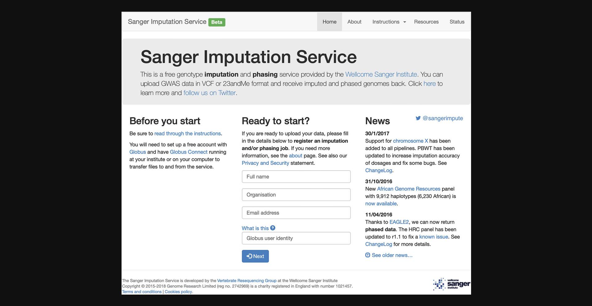
3.Navigate to the SIS homepage to upload VCF file for imputation (https://imputation.sanger.ac.uk).
4.Download the imputed GZVCF files from the SIS (instructions can be found at https://imputation.sanger.ac.uk/?instructions=1#downloadyourdata).
5.Filter out poorly imputed genotypes to reduce uncertainty of downstream results.
Alternate Protocol 1: PROCESSING SEPARATE DATASETS COMPRISING ARRAY GENOTYPE AND WHOLE-GENOME SEQUENCING DATA
Merging WGS data with array genotype data requires special considerations. Genotype data obtained from different cohorts should only be combined using intersecting or common SNPs across all groups to avoid high rates of missing data in the final merged dataset. The high-coverage genotype data obtained from WGS has the ability to completely overlap with markers on any array. However, merging WGS and array data can be complicated by differences in genotyping technologies with a high potential for introducing batch effects. This alternate protocol, adapted from the GAWMerge protocol for combining array-based genotyping and WGS data (Mathur et al., 2022), provides instructions for preparing WGS data for merging with genotype data obtained from different array platforms.
Necessary Resources
Hardware
- A computer with as much memory (≥8 GB) and computing power as possible or access to an HPC cluster. A computer running either a 64-bit Linux-based distribution (e.g., Ubuntu) or macOS is required.
Software
- PLINK v2.0 (https://www.cog-genomics.org/plink2/)
Files
- WGS data in VCF format
- List of SNPs genotyped on one of the arrays to be merged. We suggest extracting a list of SNPs from the array with the greatest marker density. For example, in our study, we used a list of SNPs genotyped on the Illumina H3Africa array (the SNP IDs can be obtained from https://chipinfo.h3abionet.org/browse).
1.Generate the list of SNPs to be extracted from the WGS data.
2.Extract the SNP list from WGS data using PLINK and convert the output file to binary PLINK file format:
- plink --vcf input_filename.vcf --extract SNP_list.txt --make-bed --out output_filename
3.Follow QC, imputation, and post-imputation QC procedures outlined in Basic Protocol 1, steps 2 to 5.
Alternate Protocol 2: PERFORMING IMPUTATION USING A LOCAL REFERENCE PANEL
In the event that researchers have a local/personalized reference panel for imputation or do not wish to use a remote imputation server, phasing and imputation can be performed by the researcher on an HPC cluster. This alternate protocol provides instructions for phasing and imputation using Eagle (Loh et al., 2016) and Minimac4 (Howie et al. 2012), respectively. This protocol follows from the genotype QC procedures outlined in Basic Protocol 1, steps 1 and 2.
Necessary Resources
Hardware
- A computer with as much memory (≥8 GB) and computing power as possible or access to an HPC cluster. A computer running either a 64-bit Linux-based distribution (e.g., Ubuntu) or macOS is required.
Software
- PLINK v2.0 (https://www.cog-genomics.org/plink2/)
- Eagle v2.4.1 (phases genotypes prior to imputation: https://alkesgroup.broadinstitute.org/Eagle/#x1-30002)
- Minimac4 (https://github.com/statgen/Minimac4)
- BCFTOOLS v1.9 (https://samtools.github.io/bcftools/howtos/install.html)
Files
- Reference genetic map files (included in the Eagle software download)
- Phased reference genotypes in tabix-indexed VCF format
1.Split target and reference VCFs into individual chromosome files using PLINK:
-
for i in {1..22}; do plink --vcf TargetSamples.vcf --chr
{i}; done -
for i in {1..22}; do plink --vcf ReferenceSamples.vcf --chr
{i}; done
2.Phase target per-chromosome VCFs using Eagle and the phased reference VCF:
- for i in {1..22}; do Eagle_v2.4.1/eagle --noImpMissing --vcfOutFormat=z --vcfTargetTargetSamples _chr
{i}.phased --vcfRef ReferenceSamples_chr${i}.vcf; done
3.Impute missing genotypes in phased target per-chromosome VCFs using Minimac4 and the phased reference VCF:
- for i in {1..22}; do minimac4 --refHaps ReferenceSamples_chr
{i}.phased.vcf.gz --allTypedSites --cpus 10 --prefixTargetSamples_imputed_chr${i}; done
Basic Protocol 2: MERGING SEPARATE DATASETS
Only intersecting or common SNPs across all separate datasets should be combined to avoid high rates of SNP missingness in the final merged dataset. This protocol describes the process of identifying and extracting intersecting SNPs from each genotype dataset, combining the separate datasets, and conducting post-merging QC procedures, such as removing duplicate or closely related individuals. In this protocol, KING software is used to identify closely related individuals. Users should familiarize themselves with the software user guide prior to beginning this protocol to understand the files generated by KING and the kinship coefficients used to estimate relatedness (https://www.kingrelatedness.com/manual.shtml).
Necessary Resources
Hardware
- A computer with as much memory (≥8 GB) and computing power as possible or access to an HPC cluster. A computer running either a 64-bit Linux-based distribution (e.g., Ubuntu) or macOS is required.
Software
- Java v1.8 (to run the Picard toolset; can be obtained from https://www.oracle.com/java/technologies/downloads/)
- PLINK v2.0 (https://www.cog-genomics.org/plink2/)
- KING v2.3.2 (https://www.kingrelatedness.com/Download.shtml)
Files
- Reference sequence FASTA file (the target sequence for the required genomic build coordinates; can be obtained from https://hgdownload2.soe.ucsc.edu/downloads.html#human)
- UCSU chain file to guide genomic coordinate conversion from one genome build to another (can be obtained from http://hgdownload.soe.ucsc.edu/downloads.html#liftover)
1.If required, convert genomic positions to the same coordinate system (e.g., hg19, hg38).
- java -jar picard.jar LiftoverVcf
- I=input.vcf
- O=lifted_over.vcf
- CHAIN=b37tohg38.chain
- REJECT=rejected_variants.vcf
- R=reference_sequence.fasta
2.Remove poorly imputed genotypes (see Basic Protocol 1, step 5) and convert imputed VCF files to binary PLINK file format:
- plink --vcf filename.vcf --make-bed --out filename
3.Screen for duplicate or closely related individuals within each separate dataset using KING software.
- king -b input_filename.bed --ibdseg
One individual from each relationship pair identified should be chosen to be removed from the dataset. The remove_relatives.py script(developed as part of the PONDEROSA algorithm; https://github.com/williamscole/PONDEROSA/tree/master) compiles a list of unrelated individuals, given the .seg file generated by the above KING command and the .fam file from PLINK. For example, pairs of individuals who are less than second-degree relatives will be identified in the following command:
- python remove_relatives.py None king.seg input_filename.fam 2nd
Use PLINK and the output list of unrelated individuals to filter related individuals from the dataset:
- plink --bfile input_filename --keep unrelated_individuals.txt --make-bed --outoutput_filename
Repeat this procedure for each separate dataset.
4.Convert all SNP positions to chromosome:basepair format using PLINK:
- plink --bfile input_filename --set-all-var-ids @:# --make-bed --out output_filename
Then, extract a list of SNPs in each dataset:
- awk ‘{print $2}’ input_filename.bim | sort > SNP_list.txt
5.Compare the SNP lists from all datasets to identify common or intersecting sites.
- comm -12 SNP_list_1.txt SNP_list_2.txt |
- comm -12 - SNP_list_3.txt |
- comm -12 - SNP_list_4.txt > Intersecting_SNPs_allDatasets.txt
6.Extract intersecting SNPs from each dataset:
- plink --bfile input_filename --extract Intersecting_SNPs_allDatasets.txt --make-bed --out output_filename
7.Use PLINK to merge the intersecting SNPs from each dataset.
8.After merging, apply additional QC steps to remove residual genotyping errors in SNPs and samples with low genotype call rates. Remove all individuals missing >10% genotypes, exclude markers with >5% missing data, and apply an HWE filter to controls (threshold < 0.00001):
- plink --bfile Merged_files --geno 0.05 --mind 0.1 --hwe 0.00001 --make-bed --out Merged_files_QC
9.As duplicate or related individuals may exist across different datasets, identify IBD segments and individuals in relationship pairs (such as parent/offspring or sibling pairs) using KING:
- king -b input_filename.bed --ibdseg
Choose one individual from each relationship pair identified to be removed from the dataset.
Sample Data
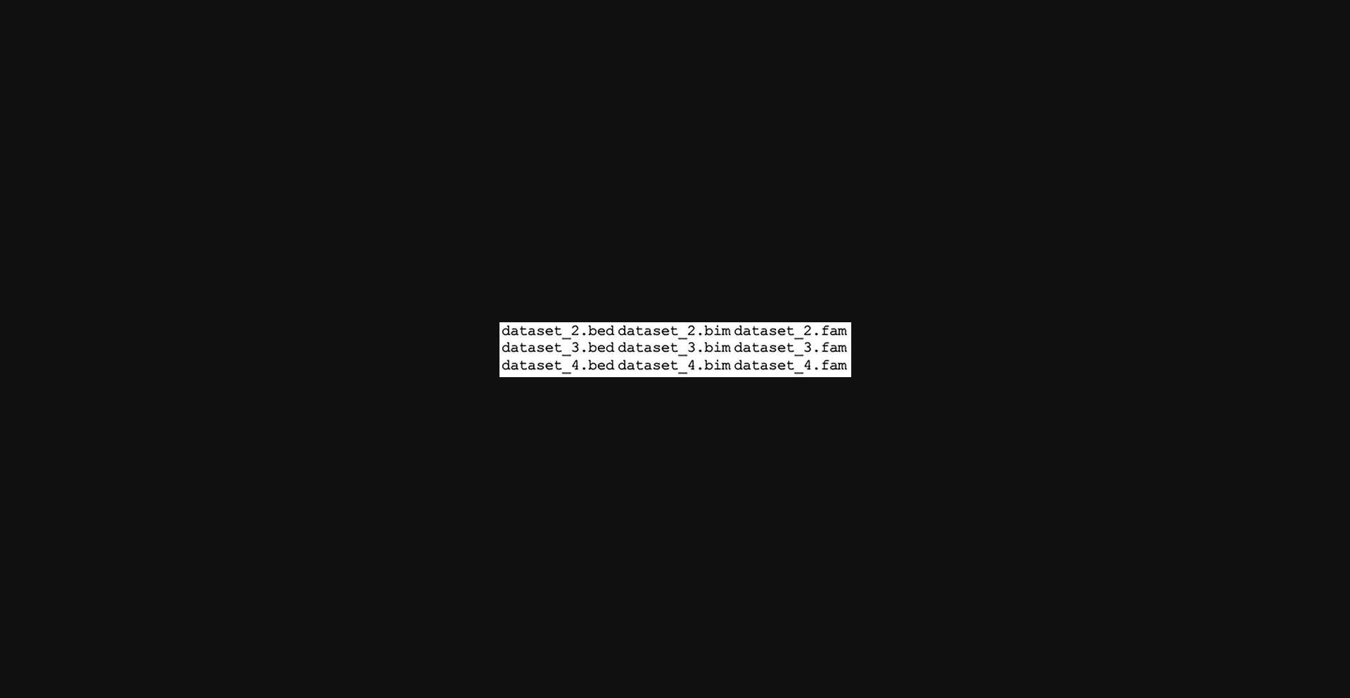
For sample data, see a list of files to be merged in Figure 2.
Basic Protocol 3: ANCESTRY INFERENCE USING ADMIXTURE AND RFMix
Population stratification (allele frequency differences between cases and controls due to differences in population structure) may confound association signals between genotype and phenotype (see Current Protocols article: Hellwege et al., 2017). Although controlling for population structure is a routine procedure in GWASs and other downstream analyses, it is particularly important when working with genotype data obtained from admixed individuals, whose ancestry is highly heterogeneous across the genome (Swart et al., 2021). Although principal components (PCs) are commonly included as covariables in GWASs to control for population structure, PCs cannot reliably deconvolute recent population structure present in complex, highly admixed populations (Elhaik, 2022). PC analysis (PCA) appropriately captures older population deviation (i.e., separation among continental population groups) (Patterson et al., 2010). However, more recent population structure (i.e., recent admixture among population clusters) cannot accurately be discerned from PCA (Petersen et al., 2013). Calculating contributing ancestral proportions is a superior method to PCA to account for population stratification in samples with recent admixture. This protocol provides instructions for estimating global ancestry proportions for individuals in the merged dataset generated by Basic Protocol 3.First, we illustrate how to produce a file of reference sample individuals and how to run the ADMIXTURE (Alexander & Lange, 2011) ancestry inference software. In this protocol, ADMIXTURE is run in an unsupervised manner to first determine the correct number of source populations contributing to the overall study population structure. Thereafter, ADMIXTURE is used to determine the global ancestry proportions of each sample. As always, users should familiarize themselves with the software user documentation prior to beginning this protocol (https://dalexander.github.io/admixture/admixture-manual.pdf). The second half of this protocol describes how to use RFMix to infer global ancestry proportions given the number of source populations determined in the first half of the protocol. Users should familiarize themselves with the RFMix user documentation (https://github.com/slowkoni/rfmix/blob/master/MANUAL.md) before beginning this protocol. Although the ADMIXTURE algorithm is perhaps the most common method of ancestry inference, RFMix (Maples et al., 2013) has been shown to outperform ADMIXTURE in determining global ancestry proportions in complex multi-way admixed populations (Uren et al., 2020). Additionally, Basic Protocol 4 requires RFMix output files. It is important to note that RFMix does not determine the correct number of contributing source populations (i.e., K). Thus, we recommend that researchers use ADMIXTURE to determine K, followed by RFMix to refine the global ancestry fractions. ADMIXTURE and RFMix have been routinely applied to complex multi-way admixed samples with success in our experience; thus, they are our software of choice for ancestry inference in populations with complex admixture patterns.
Necessary Resources
Hardware
- A computer with as much memory (≥8 GB) and computing power as possible or access to an HPC cluster. A computer running either a 64-bit Linux-based distribution (e.g., Ubuntu) or macOS is required.
Software
- PLINK v2.0 (https://www.cog-genomics.org/plink2/)
- ADMIXTURE v1.3 (https://dalexander.github.io/admixture/download.html)
- PONG v1.5 (https://github.com/ramachandran-lab/pong/tree/master)
- SHAPEIT v2 (https://mathgen.stats.ox.ac.uk/genetics_software/shapeit/shapeit.html)
- VCFTOOLS v0.1.17 (https://vcftools.github.io/index.html)
- RFMix v2 (https://anaconda.org/bioconda/rfmix)
Files
- Reference sample individuals
- Genetic map files
- Sample map file
1.Prepare a reference file.
2.Concatenate per-chromosome imputed files using BCFTools to produce one VCF (containing all chromosomes and individuals):
- bcftools concat
- ALL.chr*.phase3_shapeit2_mvncall_integrated_v5a.20130502.genotypes.vcf.gz
- -Oz -o allChromosomes_1000G.vcf.gz
3.Extract individuals from specific population groups using PLINK:
- plink --vcf allChromosomes_100G.vcf.gz --keep Populations_required.txt --make-bed --outallChromosomes_1000G_PopulationsRequired
4.Merge reference sample file and target sample file using steps outlined in Basic Protocol 2, steps 2 to 7.
5.Remove redundant SNPs through LD-pruning. Perform LD-pruning by removing each SNP with r2 > 0.1 within a 50-SNP sliding window (advanced by 10 SNPs at a time) using PLINK:
- plink --bfile TargetSamples_ReferenceSamples_Merged --indep-pairwise 50 10 0.1
Remove plink.prune.out file from target and reference merged dataset:
- plink --bfile TargetSamples_ReferenceSamples_Merged --exclude plink.prune.out --make-bed --out TargetSamples_ReferenceSamples_Merged_LD-pruned
6.Determine the correct number of ancestral/source populations contributing to the target population. Implement ADMIXTURE's unsupervised clustering algorithm with CV for a range of K values (e.g., K=3-10), where the number of contributing ancestries/populations is denoted by K:
- for k in {3..10}; do admixture --cv TargetSamples_ReferenceSamples_Merged_LD-pruned.bed
{k}; done
Inspect the log files to identify the value of K (number of contributing sourcepopulations) with the lowest CV error:
- grep -h CV log*.out
Perform 10 iterations with the correct K value to refine global ancestryproportions:
- for i in {1..10}; do admixture --cv TargetSamples_ReferenceSamples_Merged_LD-pruned.bed K -j4; done
Visualize global ancestry proportions for each individual using PONG:
- pong -m filemap -n pop_order -I ind2pop
7.Split the target and reference merged dataset into separate chromosomes before phasing:
- for i in {1..22}; do plink --bfile TargetSamples_ReferenceSamples_Merged --chr
{i}; done
8.Phase each chromosome separately using SHAPEIT:
- for i in {1..22}; do shapeit --input-bed TargetSamples_ReferenceSamples_Merged_chr
{i}.bim TargetSamples_ReferenceSamples_Merged_chr {i}.txt--ouput-haps TargetSamples_ReferenceSamples_Merged_chr${i}.haps; done
9.Convert phased files to VCF file format:
- for i in {1..22}; do shapeit -convert --input-haps TargetSamples_ReferenceSamples_Merged_chr
{i}.vcf;done
10.Prepare reference and target files required for RFMix, which requires one text file listing the sample IDs for all target individuals and one text file listing the sample IDs for all reference individuals:
-
for i in {1..22}; do vcftools --vcf TargetSamples_ReferenceSamples_Merged_chr
{i}.vcf; done -
for i in {1..22}; do vcftools --vcf TargetSamples_ReferenceSamples_Merged_chr
{i}.vcf; done
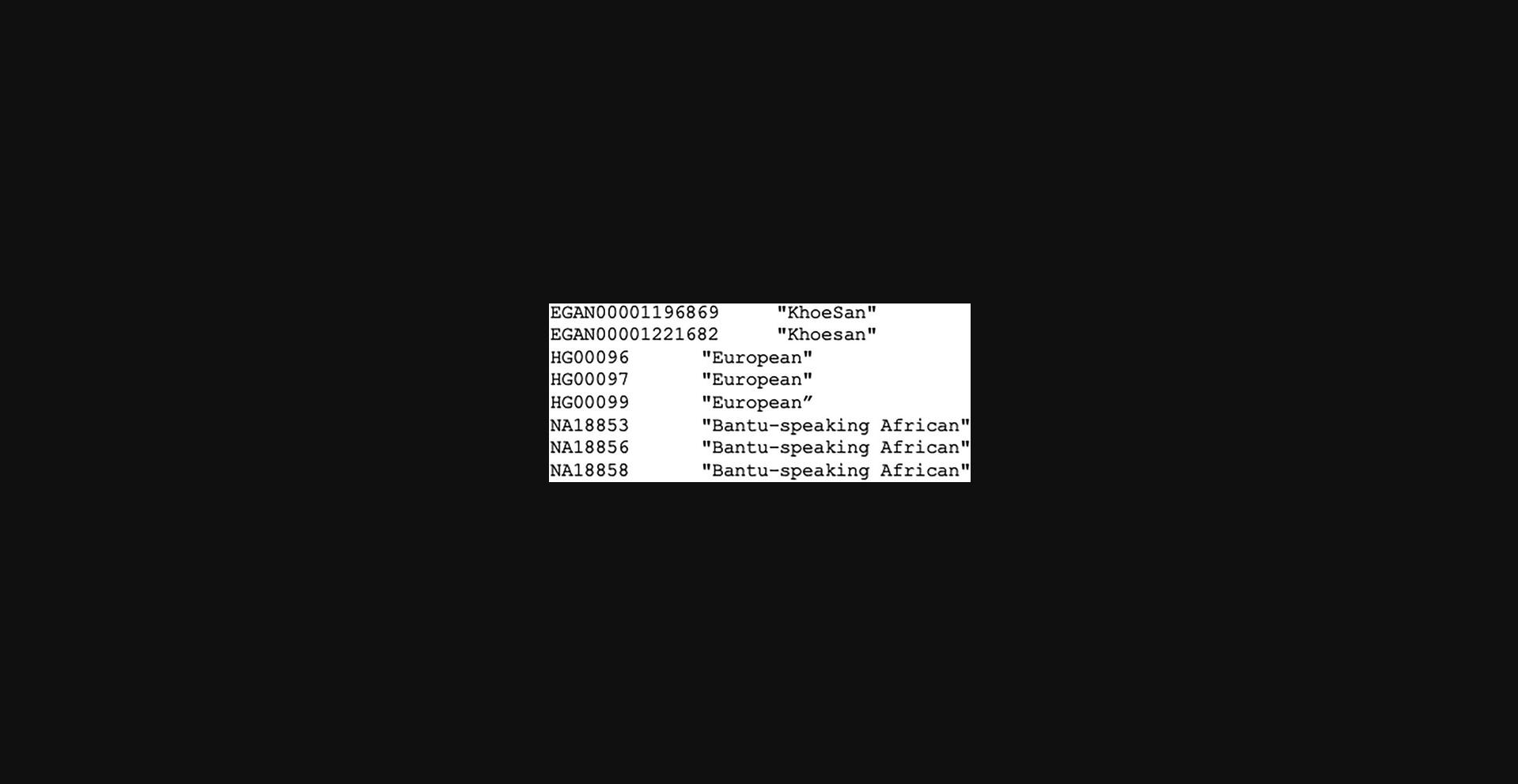
11.Create the sample map file required for RFMix.
12.Run RFMix using default parameters:
- for i in {1..22}; rfmix -f TargetSamples_chr
{i}.vcf -mSample_map -g genetic_map_GRCh37_chr {i} --reanalyze-reference-o RFMix_outputfile_chr${i}; done
Sample Data
See the sample map file required for RFMix in Figure 3.
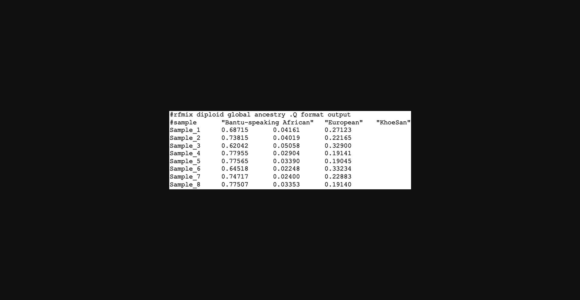
RFMix outputs global ancestry proportions for each individual in the .Q file (Fig. 4).
Basic Protocol 4: BATCH EFFECT CORRECTION USING PSEUDO-CASE-CONTROL COMPARISONS
Basic Protocol 4 described the pseudo-case-control comparison method for batch effect correction, adapted from prior work (Chen et al., 2022). This method involves coding case/control status by batch followed by running a logistic regression analysis testing each batch against all other batches. For example, the status of all samples from one dataset is coded as a case, whereas the status of every other sample is coded as a control. A logistic regression test is then performed. This procedure is repeated for each batch. If any single dataset has more positive signals compared to the other datasets, then batch effects may be responsible for producing spurious results. If batch effects are present, the genomic inflation factor (λ) for the pseudo-case-control comparisons will be greater than one. Batch effects can be resolved by removing those SNPs that pass the threshold for significant from the merged dataset, as these SNPs are affected by batch effects. The standard genome-wide threshold for significance (5 × 10⁻⁸) may be overly stringent for samples obtained from admixed populations. The R package STEAM (Significance Threshold Estimation for Admixture Mapping) (Grinde et al., 2019) calculates a less-stringent significance threshold for analyses using admixed population, taking the global ancestry proportions and number of generations since admixture into account.
Necessary Resources
Hardware
- A computer with as much memory (≥8 GB) and computing power as possible or access to an HPC cluster. A computer running either a 64-bit Linux-based distribution (e.g., Ubuntu) or macOS is required.
Software
- PLINK v2.0 (https://www.cog-genomics.org/plink2/)
- R v4.3.1 (https://www.r-project.org)
Files
- Merged target PLINK binary files (Merged_files_QC)
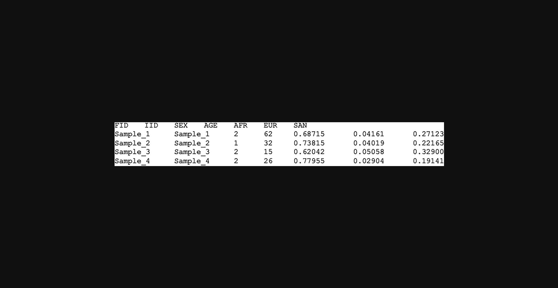
- Covariate file (Fig. 5)
1.Create a covariate file for the merged dataset.
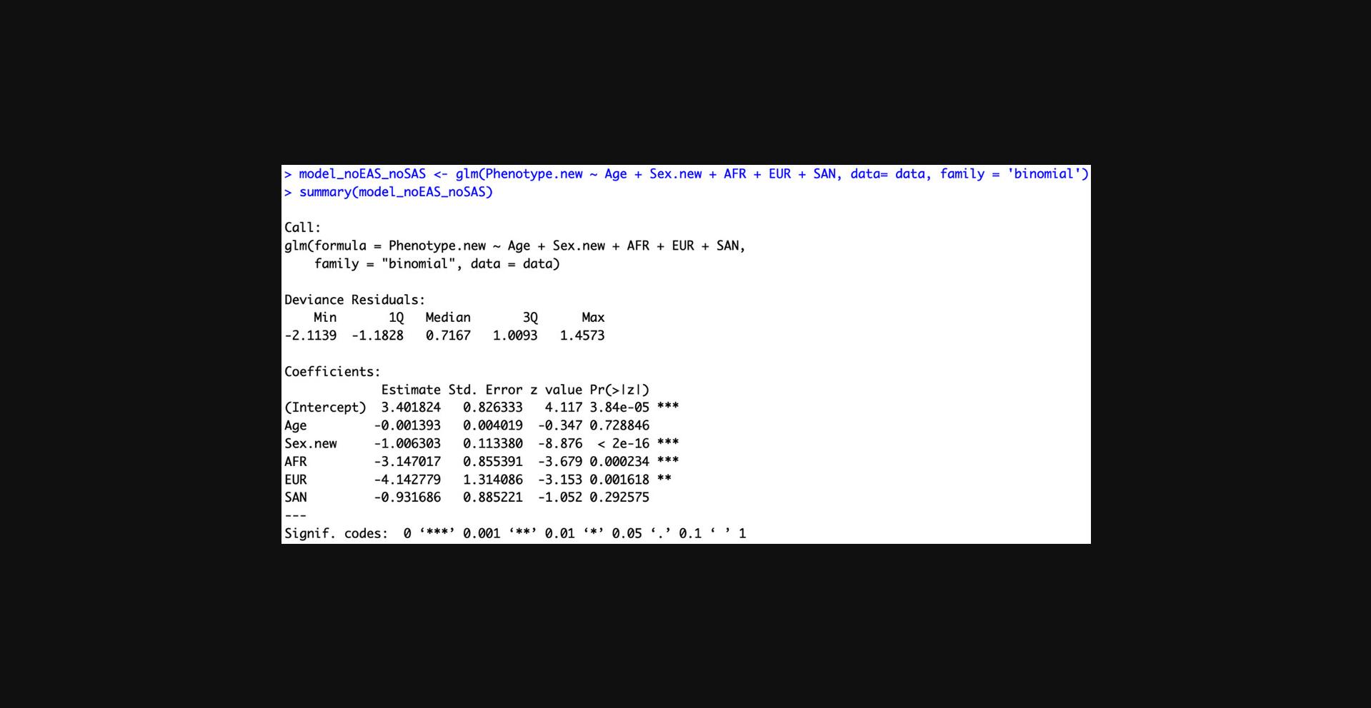
2.Determine the covariates that have the greatest effect on the outcome, which can be done by running a logistic regression test in R using the covariate file:
- R
-
Model
-
Read data
- data <- read.table("Covariates_data.txt")
- View(data)
- colnames(data) <- c("FID", "IID", "Phenotype", "Sex", "Age", "AFR", "EAS", "EUR", "SAN", "SAS")
-
Recode Phenotype (control=0, case=1)
- data
Phenotype ==1, yes=0, no=1) -
Recode Sex (male=0, female=1)
- data
Sex==1, yes=0, no=1) -
Run logistic model
- model <- glm(Phenotype.new ∼ Age + Sex.new + AFR + EUR + SAN, data= data, family = ‘binomial’)
- summary(model)
Select the covariates that have significant Z-scores (Fig. 6).
3.Because the standard genome-wide threshold for significance (5 × 10⁻⁸) might be overly stringent for samples obtained from admixed populations, calculate a new genome-wide threshold, which takes global ancestry proportions into account. Determine the genome-wide significance threshold value using STEAM.
- R
-
Install and load STEAM package
- library(devtools)
- install_github("kegrinde/STEAM")
- library(STEAM)
-
Read data
- p <- read.table(“Admixture_propostions.txt”)
- m <- read.table(“Map_file.txt”)
-
Calculate new genome-wide significance threshold
- get_thresh_simstat(g = 15, map = m, props = p, nreps = 10000)
4.Improve the stability of the logistic regression test by removing SNPs with MAF < 1%:
- plink --bfile Merged_files_QC --maf 0.001 --make-bed --out Merged_files_QC_maf
5.Code one batch/dataset as case (2) in the .fam file. Code all other batches/datasets as controls (1).
6.Run logistic regression model (use sex, age, and global ancestry proportion covariates) using PLINK:
- plink --bfile Batch1_vs_others --glm sex --covar Covariates.txt --covar-name AGE,AFR,EUR,SAN --covar-variance-standardize --adjust --ci 0.95 --out Batch1_vs_others
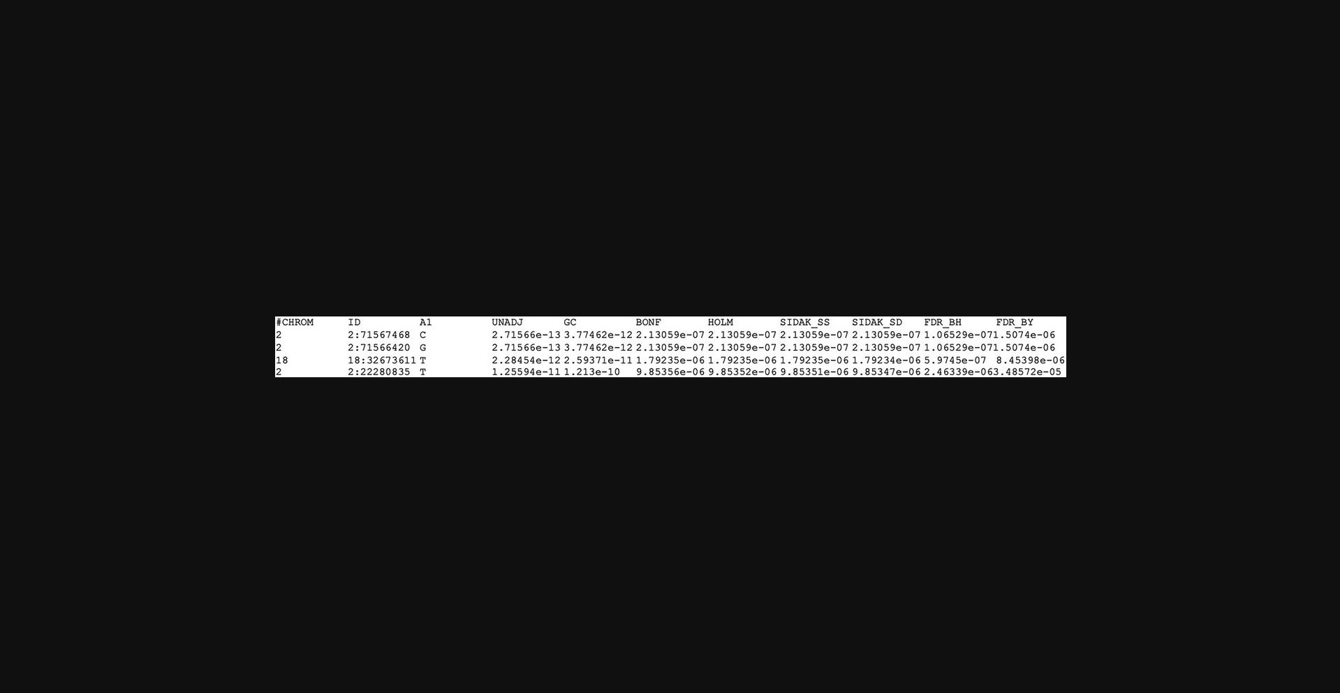
7.Inspect the Batch1_vs_others.PHENO1.glm.logistic.hybrid.adjusted output file (Fig. 9). Create a list of SNPs with Benjamini-Hochberg p -values less than the significance value calculated by STEAM.
8.Repeat steps 4 to 7 for each batch/dataset.
9.Exclude the list of SNPs affected by batch from the merged dataset:
- plink --bfile Merged_files_QC --extract BatchEffectedSnps.txt --make-bed --out Merged_files_QC_BatchEffectCorrected
Sample Data
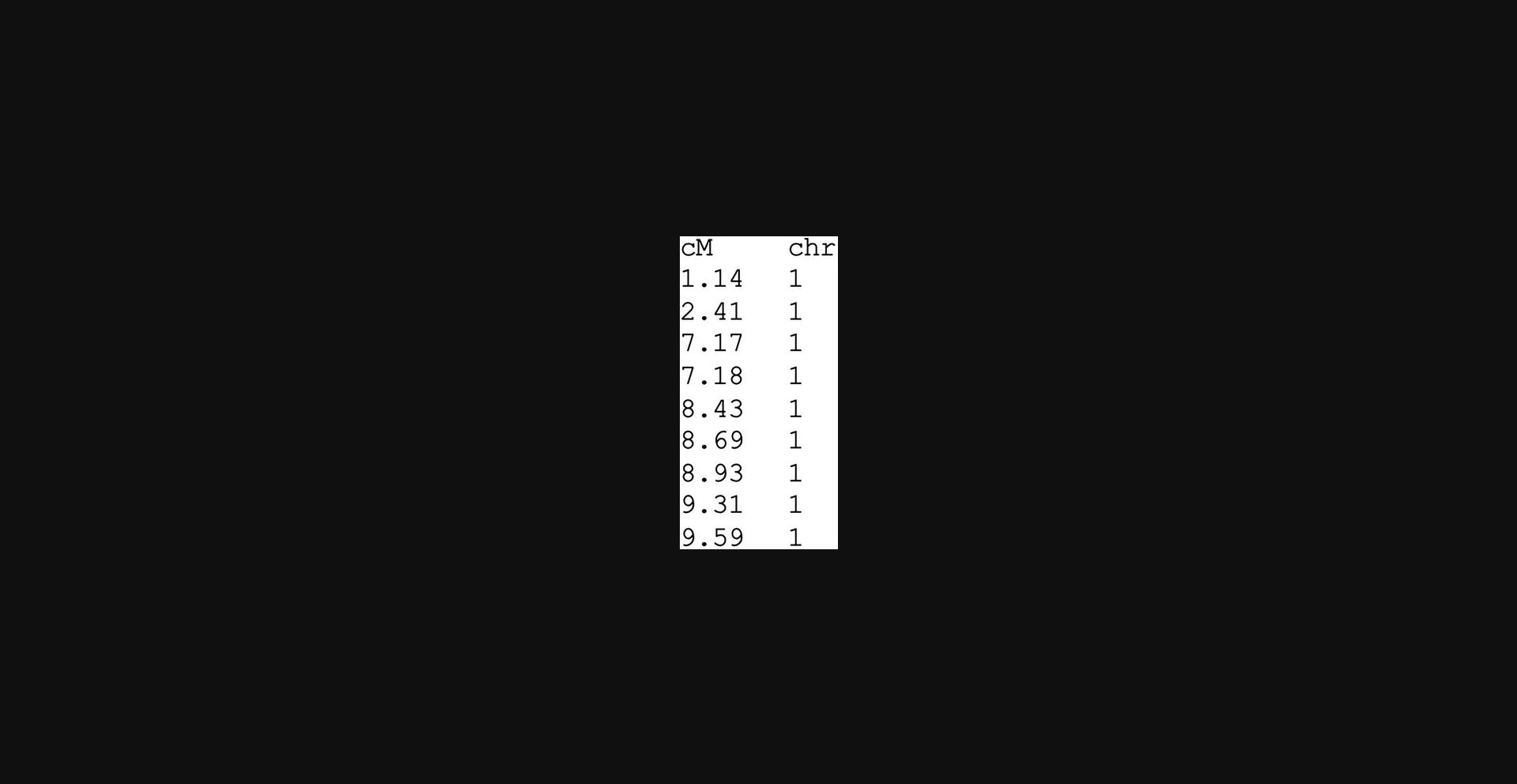
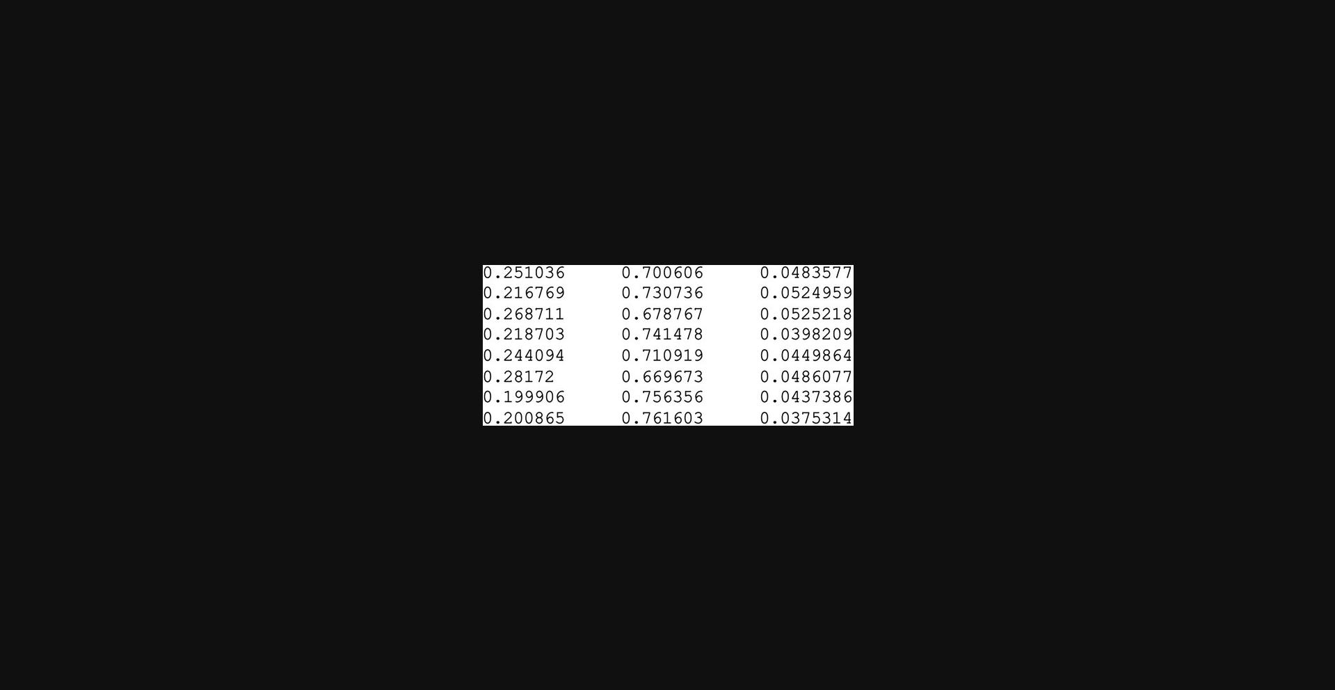
Sample data include a header of an example of a covariate file required for Basic Protocol 4 (Fig. 5), the results of a logistic regression test to determine which covariates have the greatest effect on the outcome (Fig. 6), a header map file generated from columns 1 and 4 of .msp.tsv RFMix output file (Fig. 7), the header of the admixture proportion file required for running STEAM (Fig. 8), and the header of the logistic regression output file with adjusted p-values generated by PLINK (Fig. 9).
Guidelines for Understanding Results
A logistic regression association test can be performed to determine if the data harmonization procedures were successful. Quantile-quantile (QQ) plots can be constructed to quantify the degree of inflation and determine if residual technical artifacts are confounding results.
COMMENTARY
Background Information
Data harmonization is a feasible strategy to increase sample sizes and improve the power of GWASs and other association tests. We have applied these protocols to merge separate genotype datasets without introducing spurious associations caused by batch effects or other technical artifacts. We combined six case-control genome-wide datasets [comprising five-way admixed South African Colored (SAC) individuals] to investigate host genetic variants associated with tuberculosis (TB) susceptibility. These datasets had been individually analyzed with little success, and we hypothesized that by combining these datasets, we could identify novel TB host genetic associations or confirm known associations. We applied our data harmonization guidelines for merging genotype data obtained from admixed individuals to produce a harmonized, high-quality dataset comprising 1544 individuals (952 TB cases and 592 healthy controls) free from technical artifacts. We then applied the local ancestry adjusted allelic association (LAAA) model (Duan et al., 2018) to identify ancestry-specific genetic variants associated with TB susceptibility. One SNP (rs74828248), located on chromosome 20q13.33, was significantly associated with TB susceptibility while adjusting for Bantu-speaking African local ancestry (p -value = 2.272 × 10⁻⁶, OR = 0.316, SE = 0.244). A suggestive association peak in the HLA-II region was also identified using the LAAA model while adjusting for KhoeSan ancestry. This association signal has previously been observed in a TB meta-analysis conducted by the International Tuberculosis Host Genetics Consortium (Schurz et al., 2022) and in an independent study conducted in a South African cohort (Chihab et al., 2023). Moreover, we achieved greater power to identify statistically significant markers using our harmonized dataset compared to previous analyses. Given our sample size of 1544 participants, we had a 95% chance to correctly reject the null hypothesis for markers with effect sizes from 0.2. A previous study performed by Swart et al. (2021) had a 95% chance to correctly reject the null hypothesis for large (>0.5) and medium (>0.3) effect sizes using a sample size of 735 participants from the same population group. Hence, our data harmonization guidelines have been applied to real biological data and have been shown to improve the power of downstream analyses without confounding results.
Data harmonization is necessary for large consortia that recruit thousands of samples over a period of time and require several different laboratories and facilities for genotyping and data processing. Additionally, these procedures can be employed by smaller projects to leverage external controls from public databases and make use of valuable data that may otherwise have been excluded from the analyses. However, data harmonization strategies are not widely adopted due to the challenges that arise from merging data. Guidelines for these strategies are scarce and often conflicting. For example, PCA is frequently recommended as a batch effect correction strategy despite its limited capacity to distinguish batch effects from population structure (Leek et al., 2010; Nyamundanda et al., 2017; Reese et al., 2013). Complicated procedures like data harmonization should have well-documented, robust guidelines for reproducible results. As part of this article, we present the first guidelines for merging genome-wide genotype data obtained from multi-way admixed populations. Our data harmonization strategy involves the following four steps:
Processing individual datasets (Basic Protocol 1)
Individual datasets should be processed separately at first, using standard QC procedures in which samples with high rates of missingness and variants with low genotype call rates are removed. Datasets are QC'd and imputed separately to achieve the greatest number of intersecting sites with high imputation quality across all datasets. Following QC, individual datasets should be phased and imputed separately. Poorly imputed sites should be removed to limit uncertain genotypes in downstream analyses, which could cause spurious associations.
Merging separate datasets (Basic Protocol 2)
Following post-imputation QC, separate datasets can be merged. Only sites common across all datasets should be merged. This will facilitate the merging process and ensure markers included in downstream analyses are consistent across all datasets, thereby limiting the potential for spurious associations. Additional QC procedures can be applied after merging, such as the removal of related individuals.
Ancestry inference (Basic Protocol 3)
Global ancestry proportions should be estimated using ancestry deconvolution software (like ADMIXTURE or RFMix). Global ancestry proportions should be included in null GWASs when correcting for population stratification and to account for the variation in ancestral contributions across all admixed individuals.
Batch effect correction (Basic Protocol 4)
The pseudo-case-control comparison method for batch effect correction proposed by Chen et al. (2022) can effectively be applied to admixed individuals. However, we recommend the inclusion of global ancestry proportions as covariates in place of PCA to account for differences in population structure among individuals.
These data harmonization guidelines employ thorough QC procedures to remove technical artifacts as well as uncertain genotypes following imputation and correct for the presence of batch effects in a merged dataset. Because multiple genotyping arrays are available for use in human genetic studies and new arrays are continuously being developed, data harmonization procedures that make use of imputation are essential to allow merging of disparate genotype arrays. This harmonization procedure for merging genotype data from multiple sources can be employed for other applications where individual-level genotype information is required.
Although packaged software pipelines are appealing to researchers for efficient workflows, we have chosen to not package these guidelines into a software program. Admixed populations are highly diverse with respect to their contributing ancestries. Hence, we believe that being able to tailor the guidelines to a unique population group is an advantage of an unpackaged set of guidelines, in which the researcher can adapt the thresholds and reference panels to suit their population under study.
Critical Parameters
Factors that influence the protocols and to which special attention should be paid are as follows:
Imputation reference panel (Basic Protocol 1)
As haplotype structures across different populations vary and imputation accuracy is dependent on the adequate matching of individual haplotypes to a reference, it is important to use haplotype reference panels that are matched to the population under study (Schurz et al., 2019; Sengupta et al., 2023).
Reference samples included for ancestry inference (Basic Protocol 3)
Similarly, ancestry inference accuracy is dependent on the adequate matching of target samples to reference individuals with similar haplotype structure. Thus, it is important to use reference samples that are obtained from population groups that are either similar to or at least proxies of the ancestral populations of the target samples under study. Appropriate reference populations can be selected based on the demographic history of the population under study.
Troubleshooting
Some potential problems and their respective solutions are presented in Table 1.
| Problem | Solution |
|---|---|
| Merging datasets—multiple incongruent sites | Ensure all datasets are aligned to the same assembly of the reference human genome. Datasets aligned to different versions can be lifted over using the GATK LiftoverVCF function (https://gatk.broadinstitute.org/hc/en-us/articles/360037060932-LiftoverVcf-Picard-). |
| Imputation—large proportion of low-quality genotypes | Remove sites with low INFO scores (e.g., INFO scores < 0.8) and redo the imputation procedure. The second round of imputation corrects poorly imputed genotypes, and subsequent QC of the re-imputed data should retain more high-quality sites. |
| ADMIXTURE—running groups | ADMIXTURE performs best when approximately equal numbers of reference populations and admixed populations are included. Thus, larger target datasets may need to be divided into smaller running groups with individuals from reference populations. Steps 5 and 6 from Basic Protocol 3 must be performed on each running group. |
| Phasing and RFMix—phase switching | RFMix implements a phase-correction algorithm that can cause phase switching. This is a known issue with RFMix with no straightforward solution: https://github.com/slowkoni/rfmix/issues/7. |
| GWAS—inflated results following Basic Protocol 4 | Basic Protocol 4 can be repeated using a more stringent genome-wide significance threshold if required. |
Software alternatives
Although our protocols detail steps for data harmonization using specific software, we acknowledge that researchers may wish to use other programs to achieve the same task based on their preferences and previous experience with using specific software. Alternative software for calculating relatedness and inferring ancestral proportions, which may be used to accomplish what is done in the above protocols, is presented in Table 2.
| Software | Use | Reference |
|---|---|---|
| REAP (Relatedness Estimation in Admixed Populations) | Relationship inference for admixed populations | Thornton et al., 2012 |
| RelateAdmix | Relationship inference for admixed populations | Conomos et al., 2016 |
| STRUCTURE | Global ancestry inference | Pritchard et al., 2000 |
Author Contributions
Dayna Croock : Formal analysis; investigation; methodology; writing—original draft; writing—review and editing. Yolandi Swart : Formal analysis; methodology; supervision; writing—review and editing. Haiko Schurz : Conceptualization; methodology; supervision; writing—review and editing. Desiree C. Petersen : Conceptualization; project administration; supervision; writing—review and editing. Marlo Möller : Conceptualization; data curation; project administration; resources; supervision; writing—review and editing. Caitlin Uren : Conceptualization; data curation; project administration; supervision; writing—review and editing.
Acknowledgments
We acknowledge the support of the DSI-NRF Centre of Excellence for Biomedical Tuberculosis Research, South African Medical Research Council Centre for Tuberculosis Research (SAMRC CTR), Division of Molecular Biology and Human Genetics, Faculty of Medicine and Health Sciences, Stellenbosch University, Cape Town, South Africa. We also acknowledge the Centre for High Performance Computing (CHPC), South Africa, for providing computational resources. This research was partially funded by the South African government through the SAMRC and the Harry Crossley Research Foundation.
Conflict of Interest
There are no conflicts of interest to declare.
Open Research
Data Availability Statement
No new genetic data were generated for this study. However, summary statistics for the quality and accuracy assessment of the genetic data will be made available to researchers who meet the criteria for access after application to the Health Research Ethics Committee (HREC) of Stellenbosch University. Requests to access these datasets should be directed to Marlo Möller, marlom@sun.ac.za.
Literature Cited
- Alexander, D. H., & Lange, K. (2011). Enhancements to the ADMIXTURE algorithm for individual ancestry estimation. BMC Bioinformatics , 12, 246. https://doi.org/10.1186/1471-2105-12-246
- Chen, D., Tashman, K., Palmer, D. S., Neale, B., Roeder, K., Bloemendal, A., Churchhouse, C., & Ke, Z. T. (2022). A data harmonization pipeline to leverage external controls and boost power in GWAS. Human Molecular Genetics , 31(3), 481–489. https://doi.org/10.1093/hmg/ddab261
- Chihab, L. Y., Kuan, R., Phillips, E. J., Mallal, S. A., Rozot, V., Davis, M. M., Scriba, T. J., Sette, A., Peters, B., Lindestam Arlehamn, C. S., & SATVI Study Group. (2023). Expression of specific HLA class II alleles is associated with an increased risk for active tuberculosis and a distinct gene expression profile. HLA : Immune Response Genetics , 101(2), 124–137. https://doi.org/10.1111/tan.14880
- Conomos, M. P., Reiner, A. P., Weir, B. S., & Thornton, T. A. (2016). Model-free estimation of recent genetic relatedness. American Journal of Human Genetics , 98(1), 127–148. https://doi.org/10.1016/j.ajhg.2015.11.022
- Delaneau, O., Howie, B., Cox, A. J., Zagury, J.-F., & Marchini, J. (2013). Haplotype estimation using sequencing reads. American Journal of Human Genetics , 93(4), 687–696. https://doi.org/10.1016/j.ajhg.2013.09.002
- Duan, Q., Xu, Z., Raffield, L. M., Chang, S., Wu, D., Lange, E. M., Reiner, A. P., & Li, Y. (2018). A robust and powerful two-step testing procedure for local ancestry adjusted allelic association analysis in admixed populations. Genetic Epidemiology , 42(3), 288–302. https://doi.org/10.1002/gepi.22104
- Elhaik, E. (2022). Principal Component Analyses (PCA)-based findings in population genetic studies are highly biased and must be reevaluated. Scientific Reports , 12(1), 14683. https://doi.org/10.1038/s41598-022-14395-4
- Gottesman, O., Kuivaniemi, H., Tromp, G., Faucett, W. A., Li, R., Manolio, T. A., Sanderson, S. C., Kannry, J., Zinberg, R., Basford, M. A., Brilliant, M., Carey, D. J., Chisholm, R. L., Chute, C. G., Connolly, J. J., Crosslin, D., Denny, J. C., Gallego, C. J., Haines, J. L., … eMERGE Network. (2013). The Electronic Medical Records and Genomics (eMERGE) Network: Past, present, and future. Genetics in Medicine , 15(10), 761–771. https://doi.org/10.1038/gim.2013.72
- Grinde, K. E., Brown, L. A., Reiner, A. P., Thornton, T. A., & Browning, S. R. (2019). Genome-wide significance thresholds for admixture mapping studies. American Journal of Human Genetics , 104(3), 454–465. https://doi.org/10.1016/j.ajhg.2019.01.008
- Hancock, D. B., Levy, J. L., Gaddis, N. C., Bierut, L. J., Saccone, N. L., Page, G. P., & Johnson, E. O. (2012). Assessment of genotype imputation performance using 1000 Genomes in African American studies. PLOS ONE , 7(11), e50610. https://doi.org/10.1371/journal.pone.0050610
- Hellwege, J. N., Keaton, J. M., Giri, A., Gao, X., Velez Edwards, D. R., & Edwards, T. L. (2017). Population stratification in genetic association studies. Current Protocols in Human Genetics , 95, 1.22.1–1.22.23. https://doi.org/10.1002/cphg.48
- Howie, B., Fuchsberger, C., Stephens, M., Marchini, J., & Abecasis, G. R. (2012). Fast and accurate genotype imputation in genome-wide association studies through pre-phasing. Nature Genetics , 44(8), 955–959. https://doi.org/10.1038/ng.2354
- Leek, J. T., Scharpf, R. B., Bravo, H. C., Simcha, D., Langmead, B., Johnson, W. E., Geman, D., Baggerly, K., & Irizarry, R. A. (2010). Tackling the widespread and critical impact of batch effects in high-throughput data. Nature Reviews Genetics , 11(10), 733–739. https://doi.org/10.1038/nrg2825
- Lee, J. S.-H., Kibbe, W. A., & Grossman, R. L. (2018). Data harmonization for a molecularly driven health system. Cell , 174(5), 1045–1048. https://doi.org/10.1016/j.cell.2018.08.012
- Loh, P.-R., Danecek, P., Palamara, P. F., Fuchsberger, C., Reshef, Y. A., Finucane, H. K., Schoenherr, S., Forer, L., McCarthy, S., Abecasis, G. R., Durbin, R., & Price, A. L. (2016). Reference-based phasing using the Haplotype Reference Consortium panel. Nature Genetics , 48(11), 1443–1448. https://doi.org/10.1038/ng.3679
- Maples, B. K., Gravel, S., Kenny, E. E., & Bustamante, C. D. (2013). RFMix: A discriminative modeling approach for rapid and robust local-ancestry inference. American Journal of Human Genetics , 93(2), 278–288. https://doi.org/10.1016/j.ajhg.2013.06.020
- Marees, A. T., de Kluiver, H., Stringer, S., Vorspan, F., Curis, E., Marie-Claire, C., & Derks, E. M. (2018). A tutorial on conducting genome-wide association studies: Quality control and statistical analysis. International Journal of Methods in Psychiatric Research , 27(2), e1608. https://doi.org/10.1002/mpr.1608
- Mathur, R., Fang, F., Gaddis, N., Hancock, D. B., Cho, M. H., Hokanson, J. E., Bierut, L. J., Lutz, S. M., Young, K., Smith, A. V., NHLBI Trans-Omics for Precision Medicine (TOPMed) Consortium, Silverman, E. K., Page, G. P., & Johnson, E. O. (2022). GAWMerge expands GWAS sample size and diversity by combining array-based genotyping and whole-genome sequencing. Communications Biology , 5(1), 806. https://doi.org/10.1038/s42003-022-03738-6
- McCarthy, S., Das, S., Kretzschmar, W., Delaneau, O., Wood, A. R., Teumer, A., Kang, H. M., Fuchsberger, C., Danecek, P., Sharp, K., Luo, Y., Sidore, C., Kwong, A., Timpson, N., Koskinen, S., Vrieze, S., Scott, L. J., Zhang, H., Mahajan, A., … Haplotype Reference Consortium. (2016). A reference panel of 64,976 haplotypes for genotype imputation. Nature Genetics , 48(10), 1279–1283. https://doi.org/10.1038/ng.3643
- Nelson, S. C., Stilp, A. M., Papanicolaou, G. J., Taylor, K. D., Rotter, J. I., Thornton, T. A., & Laurie, C. C. (2016). Improved imputation accuracy in Hispanic/Latino populations with larger and more diverse reference panels: Applications in the Hispanic Community Health Study/Study of Latinos (HCHS/SOL). Human Molecular Genetics , 25(15), 3245–3254. https://doi.org/10.1093/hmg/ddw174
- Nyamundanda, G., Poudel, P., Patil, Y., & Sadanandam, A. (2017). A novel statistical method to diagnose, quantify and correct batch effects in genomic studies. Scientific Reports , 7(1), 10849. https://doi.org/10.1038/s41598-017-11110-6
- Patterson, N., Petersen, D. C., van der Ross, R. E., Sudoyo, H., Glashoff, R. H., Marzuki, S., Reich, D., & Hayes, V. M. (2010). Genetic structure of a unique admixed population: Implications for medical research. Human Molecular Genetics , 19(3), 411–419. https://doi.org/10.1093/hmg/ddp505
- Petersen, D. C., Libiger, O., Tindall, E. A., Hardie, R.-A., Hannick, L. I., Glashoff, R. H., Mukerji, M., Indian Genome Variation Consortium, Fernandez, P., Haacke, W., Schork, N. J., & Hayes, V. M. (2013). Complex patterns of genomic admixture within southern Africa. PLoS Genetics , 9(3), e1003309. https://doi.org/10.1371/journal.pgen.1003309
- Pritchard, J. K., Stephens, M., & Donnelly, P. (2000). Inference of population structure using multilocus genotype data. Genetics , 155(2), 945–959. https://doi.org/10.1093/genetics/155.2.945
- Purcell, S., Neale, B., Todd-Brown, K., Thomas, L., Ferreira, M. A. R., Bender, D., Maller, J., Sklar, P., de Bakker, P. I. W., Daly, M. J., & Sham, P. C. (2007). PLINK: A tool set for whole-genome association and population-based linkage analyses. American Journal of Human Genetics , 81(3), 559–575. https://doi.org/10.1086/519795
- Reese, S. E., Archer, K. J., Therneau, T. M., Atkinson, E. J., Vachon, C. M., de Andrade, M., Kocher, J.-P. A., & Eckel-Passow, J. E. (2013). A new statistic for identifying batch effects in high-throughput genomic data that uses guided principal component analysis. Bioinformatics , 29(22), 2877–2883. https://doi.org/10.1093/bioinformatics/btt480
- Roshyara, N. R., Horn, K., Kirsten, H., Ahnert, P., & Scholz, M. (2016). Comparing performance of modern genotype imputation methods in different ethnicities. Scientific Reports , 6, 34386. https://doi.org/10.1038/srep34386
- Schurz, H., Müller, S. J., van Helden, P. D., Tromp, G., Hoal, E. G., Kinnear, C. J., & Möller, M. (2019). Evaluating the accuracy of imputation methods in a five-way admixed population. Frontiers in Genetics , 10, 34. https://doi.org/10.3389/fgene.2019.00034
- Schurz, H., Naranbhai, V., Yates, T. A., Gilchrist, J. J., Parks, T., Dodd, P. J., Möller, M., Hoal, E. G., Morris, A. P., Hill, A. V. S., & the International Tuberculosis Host Genetics Consortium. (2022). Multi-ancestry meta-analysis of host genetic susceptibility to tuberculosis identifies shared genetic architecture. medRxiv. https://doi.org/10.1101/2022.08.26.22279009
- Sengupta, D., Botha, G., Meintjes, A., Mbiyavanga, M., AWI-Gen Study, H3Africa Consortium, Hazelhurst, S., Mulder, N., Ramsay, M., & Choudhury, A. (2023). Performance and accuracy evaluation of reference panels for genotype imputation in sub-Saharan African populations. Cell Genomics , 3(6), 100332. https://doi.org/10.1016/j.xgen.2023.100332
- Stanaway, I. B., Hall, T. O., Rosenthal, E. A., Palmer, M., Naranbhai, V., Knevel, R., Namjou-Khales, B., Carroll, R. J., Kiryluk, K., Gordon, A. S., Linder, J., Howell, K. M., Mapes, B. M., Lin, F. T. J., Joo, Y. Y., Hayes, M. G., Gharavi, A. G., Pendergrass, S. A., Ritchie, M. D., … Crosslin, D. R. (2019). The eMERGE genotype set of 83,717 subjects imputed to ∼40 million variants genome wide and association with the herpes zoster medical record phenotype. Genetic Epidemiology , 43(1), 63–81. https://doi.org/10.1002/gepi.22167
- Swart, Y., Uren, C., van Helden, P. D., Hoal, E. G., & Möller, M. (2021). Local ancestry adjusted allelic association analysis robustly captures tuberculosis susceptibility loci. Frontiers in Genetics , 12, 716558. https://doi.org/10.3389/fgene.2021.716558
- Thornton, T., Tang, H., Hoffmann, T. J., Ochs-Balcom, H. M., Caan, B. J., & Risch, N. (2012). Estimating kinship in admixed populations. American Journal of Human Genetics , 91(1), 122–138. https://doi.org/10.1016/j.ajhg.2012.05.024
- Uren, C., Hoal, E. G., & Möller, M. (2020). Putting RFMix and ADMIXTURE to the test in a complex admixed population. BMC Genetics , 21(1), 40. https://doi.org/10.1186/s12863-020-00845-3
- Zuvich, R. L., Armstrong, L. L., Bielinski, S. J., Bradford, Y., Carlson, C. S., Crawford, D. C., Crenshaw, A. T., de Andrade, M., Doheny, K. F., Haines, J. L., Hayes, M. G., Jarvik, G. P., Jiang, L., Kullo, I. J., Li, R., Ling, H., Manolio, T. A., Matsumoto, M. E., McCarty, C. A., … Ritchie, M. D. (2011). Pitfalls of merging GWAS data: Lessons learned in the eMERGE network and quality control procedures to maintain high data quality. Genetic Epidemiology , 35(8), 887–898. https://doi.org/10.1002/gepi.20639

