Capturing and Processing Slaking Images With a Multi-Well Plate

Start with air-dried soil that was not previously sieved. It is recommended to measure at least 20 pea-sized (3 to 10 mm) aggregates per soil sample. More replication is useful for unstable soils. See Phillips et al. (submitted 2023) for more information on necessary replication.

If the soil sample is consolidated and does not have enough pea-sized aggregates, it can be sieved through a 6 mm mesh sieve to break it up.

Establish how you will count the wells (across or down) and create a spreadsheet identifying the sample in each well.

Example Document: SiteName P16_P17_P20_Time4_Samples.csv

The well plate we provided a 3D print file for has a notch in the upper left corner to identify the first column and row.

Make sure the tray is clean and dry, and the mesh is secured to the bottom (no tears or gaps).

Place an air-dried pea-sized aggregate (3-10 mm in diameter) in the center of each well.

In Microsoft Windows, type camera into search bar to find Camera app

In the Camera app, select the correct webcam by toggling the rotate camera icon in the upper right corner.

Take a reference image of the dry aggregates.

Adjust the brightness as needed to ensure strong contrast between the aggregates and the background.

Draw a light line in permanent marker around the well plate so you can return it to the same location consistently.

Carefully remove the multi-well tray from the soaking dish. Fill the dish with at least 2 cm water.

In the Camera App toggle the time lapse to 5 seconds.

Time lapse may need to be turned on in the settings of the Camera App.

Set up a timer for ten minutes and begin the time lapse. Transfer the multi-well tray with the dry aggregates to the pan filled with water. Quickly and carefully submerge the aggregates. Place them in the same location as the in the reference photo.

Let the time lapse run at a 5 second interval for the first minute of recording, then toggle the time lapse to the 10 second interval without pausing or stopping the time lapse.

Within the file directory where project data will be saved create a folder representing the sample that was tested. E.g. C:\Users\REM\Documents\SLAKES\SampleNameTime1_Depth1

Within the Samples folder create a folder for the images collected from the sample. E.g. C:\Users\REM\Documents\SLAKES\SampleNameTime1_Depth1\Images

Move the captured images to the Images folder created in step 12.1 . The default save location for the Camera app is the Camera Roll subfolder in the active user's Pictures folder. E.g. C:\Users\REM\Pictures\Camera Roll

Ensure the Camera Roll folder is empty before starting a different sample.

With ImageJ open, import the collected images. This can be done by dragging and dropping the images from the image folder created in step 12.1. The images can also be imported through ImageJ by selecting 'File' from the menu followed by 'import' and then 'Image sequence'.

If importing through the Drag and Drop method the images will need to be converted to a stack. From the menu select 'Image', 'Stacks', and 'Images to Stack'.

Navigate the image stack with the left and right arrow keys. Make sure the images are in order. Delete any images with hands or other interference in them. Through the menu select 'Image', 'Stacks' and 'Delete Slice'.

Set the Scale of the Image with the Straight Line Tool in ImageJ.

Drag the Straight Line Tool across a well plate.

In the ImageJ menu go to 'Analyze' and 'Set Scale'. Enter the measured length of the single well in the Known distance section, Change the Unit of length to mm.

Crop the image stack down to the area with just the well plate in it by selecting using the square selection tool and from the menu selecting 'Image' and 'Crop'.

Change the image stack to the 8-bit format by selecting 'Image', 'Type', and '8-bit'.

In the Menu select 'Analyze', 'Tools' and 'ROI Manager' to open the Region of Interest (ROI) Manager tool.

Use the oval or rectangle tool to select the first well.

In the ROI Manager click Add or use the T as a shortcut to add the selection to the ROI manager tool.

Check the Show All checkbox to confirm numbers and locations as you add each individual well.

Make the image stack a set of Binary images.

In the Menu select 'Process', 'Binary', and 'Make Binary'.

Images in the stack should generate a red layer over the soil aggregates. If any shadows are picked up during this stage they will also appear in red. If this happens cancel the Make Binary action and adjust the Contrast through the Menu by selecting Image then Adjust and Brightness/Contrast until shadows no longer appear in the selected ROIs.

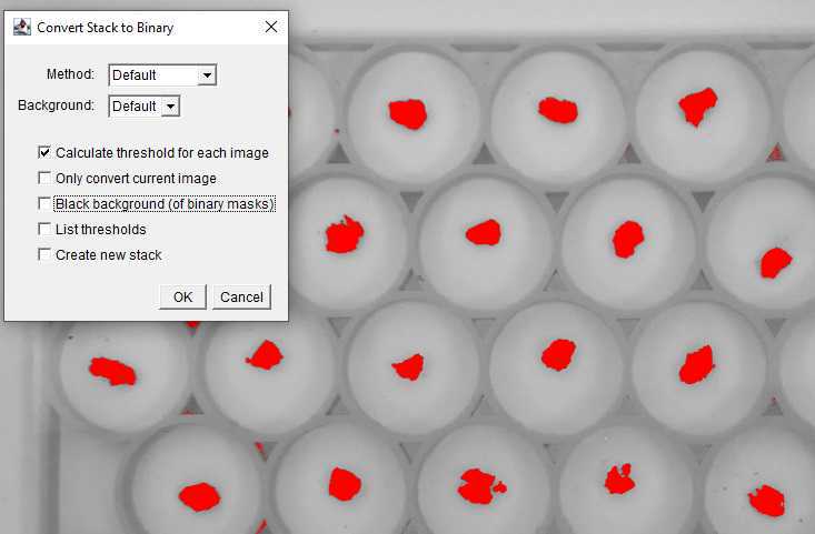
Uncheck the "Black background" box.

In the Menu select 'Analyze' then 'Set Measurements'. This will open the Set Measurements menu, which dictates what the ROI manager will analyze.

In the Set Measurements menu select Area, Stack position, and Limit to Threshold. The Redirect to dropdown should be set to None and the Decimal places box should be set to 3.

From the ROI manager window select 'More' and 'Multi Measure' to open the Multi Measure menu.

In the Multi Measure menu check the boxes for 'Measure all # Slices' and One row per slice.

Save the Multi Measure results in the sample folder created in step 12 . The filename should match the format being used with '_Results' appended at the end.

E.g. SampleNameTime1_Depth1_Results.csv

Several versions of slaking index calculations have been suggested. The slaking index originally recommended by Fajardo et al. (2016) involved fitting a rise-to-threshold (Goempertz function) model to timeseries of aggregate area, and computing the function's limit as the slaking index (SI).

Flynn et al. (2020) recommended instead computing the observed change in aggregate area over time:

     _SI600_  = ( _A600 - A0_ <sub>600</sub> - A<sub>0</sub>)/ _A0_ <sub>0</sub>

where A0 ₀ is the initial projected area of the dry aggregate and A600 ₆₀₀ is the projected

area after 600 seconds of slaking. Note that higher SI600 value indicates lower aggregate stability, as a less stable ped will spread out more over time.

By contrast, Rieke et al. (2022) reported a slaking score as 1/(1 + SI600), such that higher values indicate greater aggregate stability, which follows the same direction as other aggregate stability measures.

This R script provides example code for using the Image-J output to plot area timeseries and compute slaking index following Flynn et al. (2020). ComputeSlakingIndex.R

Slaking index tends to follow a log-normal distribution with a long right tail. Because arithmetic means are influenced by high outliers, it is recommended to use a geometric mean (and geometric standard deviation) to summarize the aggregates for each soil sample.

The geometric mean is equivalent to computing the arithmetic mean of log-transformed

data, and back-transforming the mean: .