ezTrack—A Step-by-Step Guide to Behavior Tracking
Zachary T. Pennington, Zachary T. Pennington, Keziah S. Diego, Keziah S. Diego, Taylor R. Francisco, Taylor R. Francisco, Alexa R. LaBanca, Alexa R. LaBanca, Sophia I. Lamsifer, Sophia I. Lamsifer, Olga Liobimova, Olga Liobimova, Tristan Shuman, Tristan Shuman, Denise J. Cai, Denise J. Cai
Abstract
Tracking animal behavior by video is one of the most common tasks in neuroscience. Previously, we have validated ezTrack, a free, flexible, and easy-to-use software for the analysis of animal behavior. ezTrack's Location Tracking Module can be used for the positional analysis of an individual animal and is applicable to a wide range of behavioral tasks. Separately, ezTrack's Freeze Analysis Module is designed for the analysis of defensive freezing behavior. ezTrack supports a range of desirable tools, including options for cropping and masking portions of the field of view, defining regions of interest, producing summary data for specified portions of time, algorithms to remove the influence of electrophysiology cables and other tethers, batch processing of multiple videos, and video down-sampling. Moreover, ezTrack produces a range of interactive plots and visualizations to promote users' confidence in their results. In this protocols paper, we provide step-by-step instructions for the use of ezTrack, from tips for recording behavior to instructions for using the software for video analysis. © 2021 The Authors. Current Protocols published by Wiley Periodicals LLC.
This article was corrected on 4 August 2022. See the end of the full text for details.
Basic Protocol 1 : Software environment installation
Basic Protocol 2 : Using the Location Tracking Module
Basic Protocol 3 : Using the Freeze Analysis Module
INTRODUCTION
Fundamental to the study of neuroscience is the relationship between brain and behavior. To evaluate this relationship, researchers in the field have developed increasingly sophisticated tools to probe neural function. However, the ability to measure animal behavior in an automated manner—and thus free researchers from hundreds of hours spent meticulously watching video footage—has been hindered by the high cost of software and hardware setups.
Recently, we developed ezTrack, an open-source software designed for the fast and flexible analysis of user-acquired behavioral videos (Pennington et al., 2019). ezTrack is composed of two modules that allow the analysis of a host of tests routinely deployed in neuroscience laboratories. ezTrack's Location Tracking Module (Basic Protocol 2) enables users to track an animal's location within nearly any arena, the distance it travels, and time spent in user-defined regions of interest. It can be used for a wide range of behavioral tasks, from the open field test to the radial arm maze. The Freeze Analysis Module (Basic Protocol 3) enables the measurement of defensive freezing, common to studies of both learning and defensive behavior.
Since its original publication, ezTrack has grown in popularity, owing to many of its key features (Bitzenhofer, Pöpplau, Chini, Marquardt, & Hanganu-Opatz, 2021; Bourdenx et al., 2021; Kesner et al., 2021; McCauley et al., 2020; Montanari et al., 2021; Rajbhandari et al., 2021; Shuman et al., 2020; Zeidler, Hoffmann, & Krook-Magnuson, 2020). It is free, easy to use, produces highly reliable and accurate results, contains a range of interactive data exploration/visualization tools, has a suite of functions to refine videos, and has no operating system or hardware requirements. Additionally, ezTrack has been independently validated to produce results comparable to those of commercially available software (McElroy et al., 2020). Moreover, because it is open source, researchers can modify ezTrack to suit their needs. ezTrack has also been adopted in the classroom, being a great introduction to image processing and Python programming. Although ezTrack is not without limitations (see Table 1 for an overview of its capabilities and limitations), its ability to handle many common behavioral neuroscience tests makes it an attractive option for many.
| Location Tracking Module | Freeze Analysis Module | |
|---|---|---|
| Variables calculated |
● Spatial location of animal ● Distance travelled ● Time spent in ROIs |
● Freezing ● Motion (i.e., number of frame-by-frame pixel changes) |
| Example behavioral tests |
● Elevated plus maze ● Place preference ● Open field ● Radial arm maze ● Infinity maze |
● Fear conditioning ● Forced swim test ● Diurnal activity |
| Visualization tools |
● Video playback of tracking ● Heatmaps of position ● Frame by frame distance plots |
● Video playback of tracking ● Freezing/motion plots |
| Processing tools |
● Wire-removal ● Video cropping ● Spatial down-sampling ● Masking regions from video ● Video down-sampling ● Scale conversion (e.g., pixels to inches) |
● Video cropping ● Spatial down-sampling |
| Fields of view |
● Side-view ● Top-down |
● Side-view ● Top-down (incompatible with tethers) |
| Batch processing | Yes | Yes |
| Frame-by-frame output | Yes | Yes |
| Binned summary reports | Yes | Yes |
| Tracking of multiple animals in the same arena | No | No |
| Real-time analysis | No | No |
| File types | .avi, .mkv, .mov, .mpg, .mp4, .wmv, and more | .avi, .mkv, .mov, .mpg, .mp4, .wmv, and more |
| Operating system | Windows, Linux, OSX | Windows, Linux, OSX |
In this protocols paper, we hope to further bolster the ease of getting automated behavior tracking started in a lab by providing users with a step-by-step guide to using ezTrack. This includes instructions for installing and utilizing the software (Basic Protocol 1), as well as considerations for recording behavior (see Strategic Planning). Because this is intended as an instructional tool, we refer readers to the original manuscript for details regarding the underlying algorithms and validation (Pennington et al., 2019).
STRATEGIC PLANNING
Capabilities and limitations
ezTrack enables users to perform animal tracking using two modules. The Location Tracking Module (Basic Protocol 2) allows the analysis of an animal's position in the field of view (in x ,y coordinates), the distance it travels, and its time spent in user-defined regions of interest (ROIs). The Freeze Analysis Module (Basic Protocol 3) was fundamentally designed to measure freezing for studies of defensive behavior, but could conceivably be used for any task in which motion is converted into a binary variable (e.g., swimming/not swimming in the forced swim test). Below we outline ezTrack's capabilities, as well as its current limitations.
Capabilities
The capabilities of ezTrack are summarized in Table 1.
Limitations
It is not currently possible to analyze tests involving social interactions between animals or any test where multiple animals are in the same arena. Moreover, ezTrack currently requires that the animal under study remain in the field of view for the entirety of the tracking period. ezTrack is unable to measure nuanced interactions with objects (e.g., sniffing, grabbing, burying), nor can it quantify fine motor movements. Currently, ezTrack is exclusively a post-acquisition software and cannot measure behavior in real time.
Computer, Operating System, and Browser Requirements
A major benefit of ezTrack is that it does not require specialized computer hardware; a standard laboratory desktop or personal computer is sufficient. In our laboratory, students routinely process videos on their personal laptops (e.g., a computer with 8 GB RAM and a 2.7-GHz Intel Core i5 CPU). However, when using older computers with less powerful CPUs, ezTrack's down-sampling capabilities can be used to speed processing.
ezTrack is compatible with Windows, OSX, and Linux operating systems.
ezTrack is run within a web browser, and users should take into consideration the web browser used. ezTrack has been most extensively tested, and proven to be most reliable, using Google Chrome. Multiple errors have been reported by users attempting to use Internet Explorer. Notably, although ezTrack is run within a web browser, it does not require internet access.
Recording Hardware and Video Requirements
ezTrack does not require the use of a specific camera. The only requirement is that the camera be mounted so that the field of view remains fixed for the entirety of an individual recording session. Videos captured in color or grayscale are acceptable. However, because color videos are larger in file size and still read as grayscale by ezTrack, we prefer grayscale. Moreover, because ezTrack works on previously acquired videos, any video acquisition software will work, provided that a standard video file format is produced. ezTrack can process a wide range of video file formats. The file formats so far tested include .avi, .mkv, .mov, .mpg, .mp4, and .wmv, but many more are likely compatible. ezTrack is not currently compatible with temporal compression algorithms. In the event that a particular video file format cannot be read by ezTrack, we recommend using any of the many free online softwares available for video conversion.
Processing Time Considerations
The speed at which ezTrack processes videos is entirely dependent upon the user's computer, the size of each video frame, and the physical location of video files (stored locally vs on remote drives). Nevertheless, even with modest laptops (e.g., a computer with 8 GB RAM and a 2.7-GHz Intel Core i5 CPU), ezTrack processes many videos at several-fold real time. Additionally, if a large number of videos is to be processed, batch processing can be initiated at the end of the day in order that all videos will be processed by the next morning. If the user would like to further speed processing, we offer the following recommendations:
- 1.Store videos on a local computer drive (i.e., the computer that is running ezTrack).
- 2.Use solid-state hard drives, which will speed processing.
- 3.If remote drives are to be used, connect to them via ethernet or USB. Wireless transfer is substantially slower than wired transfer.
- 4.Use ezTrack's down-sampling functions to reduce file size.
General Considerations for Recording Behavior
Below are general guidelines for recording animal behavior. Although recording strategies may vary between tasks, the following suggestions should be considered before beginning an experiment and modified as necessary for optimal results.
- 1.Choose the best suited angle of recording.
Typically, behavior is recorded either top-down or from the side. The most effective view will depend upon the arena and the variables of interest. However, for ezTrack to work effectively, the animal must be visible throughout the entirety of an individual recording session, and the camera must be in a fixed position. Top-down recording permits tracking an animal's location at all points of an arena, provides a more reliable estimate of distance traveled than side-view recording, and is sometimes more space-efficient within the laboratory. That said, this angle can be problematic when recording tethered animals, as artifacts from cables are harder to eliminate, and cannot currently be eliminated at all in ezTrack's Freeze Analysis Module. If the user is measuring freezing with tethered animals, we recommend side-view recording, as the portion of the video containing the cable can be easily cropped. Moreover, side-view recording can be helpful when researchers are interested in measuring vertical movement of the animal.
- 2.Maintain stable room lighting.
Dramatic shifts in lighting will change the background and can disrupt tracking.
- 3.Disable auto-exposure and auto-focus on the recording camera.
Auto-exposure and auto-focus mechanisms disrupt the stability of the arena background and should therefore be disabled.
- 4.Define video attributes including field of view, contrast, focus, and resolution.
Be sure to adjust the video's brightness such that there is a significant degree of contrast between the background and the subject. ezTrack will work most efficiently if the contrast between the subject and the arena is robust. If it is difficult for the experimenter to see where the animal is on the screen, ezTrack will have similar difficulty.
Be sure to set a resolution that is best fit for the video prior to recording. It is not necessary to record videos at a very high resolution. Choosing the lowest resolution in which the animal is still clearly visible will promote the fastest processing by ezTrack, and can reduce data storage burdens in the laboratory. Although choosing the lowest resolution in which the subject can still be seen will aid processing efficiency, ezTrack also has a down-sampling feature that makes processing high-definition videos more efficient.
- 5.Avoid blind spots.
It is important to angle the camera so that the animal is always visible. A simple way to test this before beginning is to place an object of similar size and color to the animal in various portions of the arena. A general rule of thumb is that if you can see the object/animal in the camera, ezTrack will be able to track it.
- 6.Be mindful of experimenter entry into the field of view.
Although ezTrack has several tools to mitigate the influence of objects other than the animal that enter the field of view, it is best to avoid this when possible. That said, if the experimenter's hands must enter the field of view, wearing gloves/clothes of similar color to the background will decrease noise and produce the most accurate data output. If the experimenter enters a portion of the field of view that does not overlap with the arena, this area can be cropped from the image using ezTrack. Lastly, ezTrack's Location Tracking Module has an additional algorithm that can reduce bias from external objects, such as hands, that briefly enter the field of view, even if they overlap with the arena. See Basic Protocol 2 for further details.
- 7.Take steps to prevent disruptions from cables or optogenetic pulses.
In many neuroscience experiments, animals are tethered, be it by recording cables, self-administration/microdialysis tubing, etc. The following recommendations will help overcome the challenges of tracking animals with cables attached.
1.If measuring freezing, users are encouraged to use side-view recording. ezTrack's wire removal algorithm has not yet been implemented in the Freeze Analysis Module, and the recommended solution is to crop out the portion of the field of view containing the wire. This is only possible with side-view recording. 2.Tethers of similar color to the background, or opposite in color to the animal, will be less disruptive to tracking. 3.When using ezTrack's wire-removal algorithm for location tracking, note that the wire must be of smaller width than the animal in the field of view. Consider the placement of the camera to promote this. If there is a portion of the tether that is of large diameter (e.g., a crane or commutator), try to exclude this from the field of view or place it in a portion of the field of view that can be later excluded from the analysis using ezTrack's cropping/masking tools. 4.Make efforts to reduce the visibility of optogenetic pulses. Many researchers accomplish this by covering dental cement on top of the animal's head with black nail polish.
NOTE : All protocols involving animals must be reviewed and approved by the appropriate Animal Care and Use Committee and must follow regulations for the care and use of laboratory animals.
Basic Protocol 1: SOFTWARE ENVIRONMENT INSTALLATION
Since the original publication of ezTrack, new features have been added. These include a wire-removal algorithm to improve the tracking of animals attached to wires or tethers, the ability to mask portions of the field of view that the user would like ignored, and functionality to down-sample videos to speed processing. To utilize these new features, and any features added subsequent to this publication, ensure that the latest ezTrack version and packages are installed. For the most up-to-date installation instructions, visit https://github.com/DeniseCaiLab/ezTrack.
Necessary Resources
Computer system (see Strategic Planning)
- Miniconda (https://docs.conda.io/en/latest/) or Anaconda (https://www.anaconda.com)
ezTrack (https://github.com/DeniseCaiLab/ezTrack)
ezTrack installation
1.Download Miniconda/Anaconda.
Installation of ezTrack requires the user to download the free package management system Miniconda or its larger counterpart Anaconda (https://www.anaconda.com). For those with minimal programming experience, using the PKG installer is likely to be more intuitive.
2.Create ezTrack environment.
After installing Miniconda/Anaconda, the user can create the ezTrack Conda environment, which will contain all of the package dependencies necessary for ezTrack to run. This is achieved by entering the following command into one's Terminal (on OSX/Linux) or Anaconda Prompt (on Windows):
conda create -y -n ezTrack -c conda-forge python=3.6 pandas=0.23.0 matplotlib=3.1.1 opencv=3.4.3 jupyter=1.0.0 holoviews=1.13.5 scipy=1.2.1 bokeh=2.1.1 tqdm
3.Download ezTrack files.
From the ezTrack Github page (https://github.com/DeniseCaiLab/ezTrack), download all files necessary to run ezTrack onto your computer: On the main page for ezTrack, click the button to “Clone or download,” and download the zip folder onto your hard drive. The unzipped folder is called “ ezTrack-master.” Alternatively, use git commands if you are familiar with them. The user should feel free to rename this folder and place it wherever they would like on their computer.
Introduction to Jupyter Notebooks
ezTrack's modules are run within what are called Jupyter Notebook files (extension .ipynb). When opened, these files contain a mixture of headings and instructions, as well as chunks of iPython code, called “cells.” When the code in a cell is executed, or “run,” relevant output such as images or plots are displayed immediately below it. Most cells of code need not be modified. When minimal alterations are necessary, instructions are provided immediately above each cell, as well as in this publication. Cells of code have been numbered, and it is assumed that the user will step through the code in order. However, there are two exceptions to this. First, some cells are marked as optional and can be skipped. Second, although the user should not skip from Cell 1 to Cell 10 without running the intervening cells, it is often useful to return to a previous step. For example, the user might first run up to Cell 8, decide they would like to tweak parameters in Cell 5, and then re-run Cells 5-8.
Below we point the reader to several pertinent features of the Jupyter Notebook files in ezTrack, which will likely be all that is needed to get started. A screenshot is provided in Figure 1, and below we describe the significance of each labeled region. We refer the reader to the internet for extensive tutorials on how to use Jupyter Notebook.
- A.The File menu.
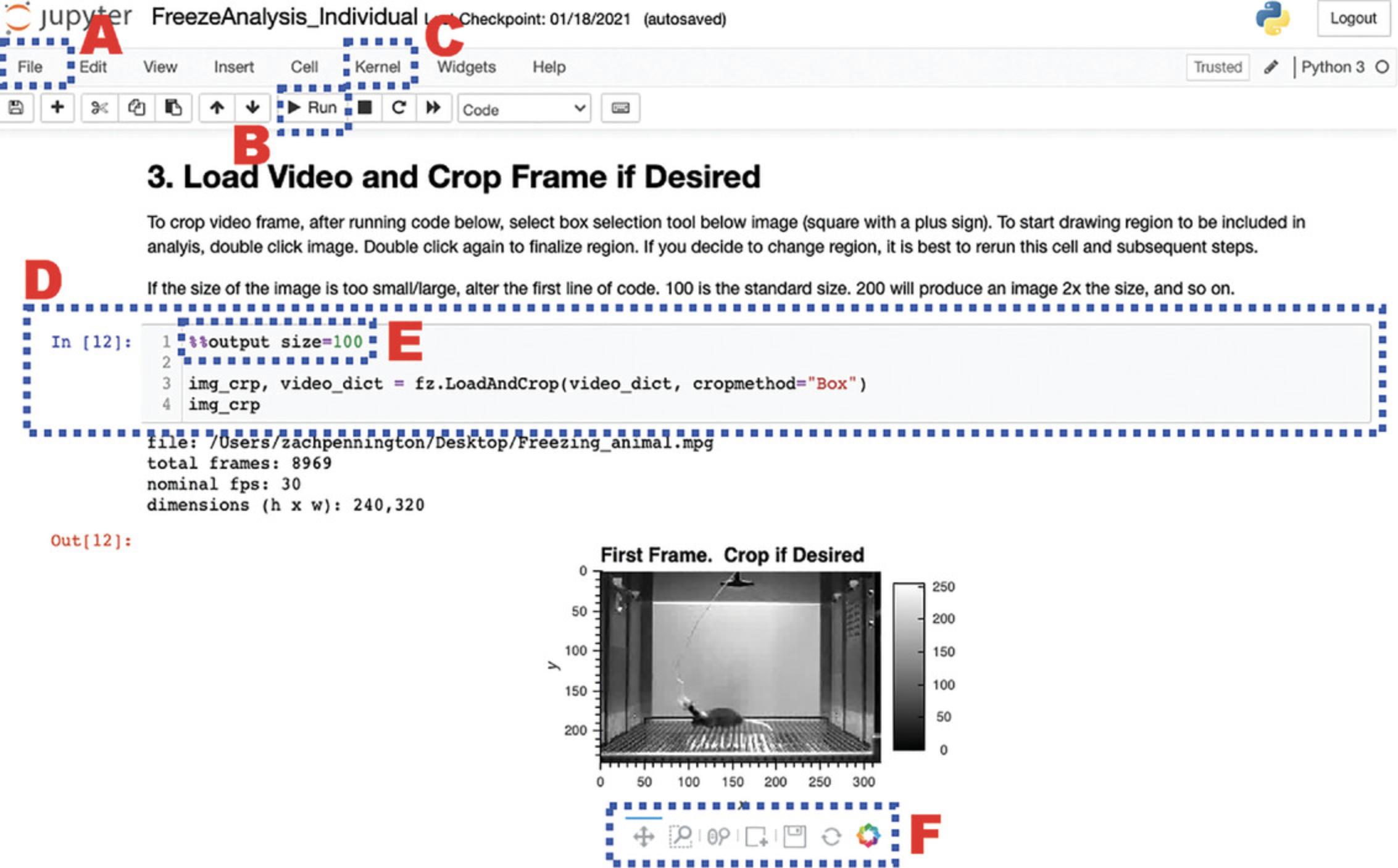
Jupyter Notebook's File menu contains several relevant options. In particular, the user can opt to print the notebook file when they are done, which allows them to save a snapshot of all their settings and the session's output. The user can also save the notebook file with a different name, such as the name of the experiment they are scoring videos from. In this way, the user can keep a more permanent record of their workflow. Note that all selected parameters will also be saved in ezTrack's .csv output files.
- B.The Run button.
After clicking on a cell of code to select it, click the Run button to execute the selected cell. Alternatively, use the shortcut, Shift + Enter.
- C.The Kernel menu.
The Jupyter Notebook Kernel holds a memory of all defined variables, loaded packages, and printed output for a session. If the user would like a clean slate, they can select Kernel, then Restart & Clear Output. All output will be removed from the notebook, and variables will be cleared from computer memory.
- D.Cells of code.
Each cell of code is visible as a gray box, and the user can change the code as they see fit. For text changes to take effect, the cell must be run. While a cell is actively being run, a “*” will appear in the brackets to the left of the cell. When complete, a number will appear, corresponding to the order in which that cell was run (e.g., if a user starts a session and runs Cell 1 twice, a 2 will appear when the code is done being executed). This helps the user track which cells they have run and in what order.
- E.Output size.
All cells of code producing image output start with the line %%output size=100. This number can be increased or decreased to change the image output size. Notably, if the dimensions of the video frame are very small in one dimension (such as on a long linear track), sometimes no image will appear. Increasing the output size to 200 or more will remedy this.
- F.Interactive image tools.
All ezTrack image output is interactive and savable. The user can use the magnifying glass with a box to select a region of an image to zoom in on. The magnifying glass with a scroll bar can be used to pan in and out (note that placing the cursor over the axis text enables the user to pan in and out selectively on that axis). The circular arrows are a refresh button. The save button allows the user to save the image as a .png file.
Basic Protocol 2: USING THE LOCATION TRACKING MODULE
ezTrack's Location Tracking Module assesses an animal's location across the course of a single, continuous session. The module can be used to calculate the amount of time an animal spends in user-defined ROIs and the distance that it travels. It uses the animal's center of mass to determine the animal's location in each frame of the video, and saves frame-by-frame location data in convenient and accessible .csv files. Summary files can also be created specifying the total distance traveled in user-defined time bins and the proportion of time in user-defined ROIs. The Location Tracking Module can be used either to process an individual video file or to process several video files in batch.
The protocol for utilizing the Location Tracking Module to analyze a single video (LocationTracking_Individual.ipynb) is outlined in detail below. This protocol provides the user with an array of visualization tools to explore parameter settings to confirm accurate tracking. We highly recommend using this protocol on a few individual videos from each experiment before proceeding to process multiple videos in batch. Given the large degree of overlap between the processing of individual files and batch processing, we will only briefly discuss batch processing (LocationTracking_BatchProcess.ipynb) and highlight the differences from individual processing.
Necessary Resources
Please see Strategic Planning regarding hardware/software considerations
Open the relevant Location Tracking file
i. Activate the ezTrack environment.
For OSX/Linux users, open a terminal. If using Windows, open Anaconda Prompt. Type the following command and then hit Enter:
conda activate ezTrack
ii. Launch Jupyter Notebook.
Within Anaconda Prompt/Terminal, type the following command and then hit Enter:
jupyter notebook
iii. Select Notebook file from Jupyter Notebook.
Within Jupyter Notebook, navigate to the folder containing the ezTrack files downloaded from the Github site, and open either LocationTracking_Individual.ipynb or LocationTracking_BatchProcess.ipynb.
Process an individual file (LocationTracking_Individual.ipynb)
Note that the numbering of the following instructions corresponds to the numbered blocks of code in the Jupyter Notebook file (called “cells”). Some of these cells are optional, as noted both here and in the Jupyter Notebook file itself.
1.Load necessary packages.
Running Cell 1 loads all necessary packages and does not need to be modified.
2.Set directory and file information, and specify ROI names, if any.
In Cell 2, the user specifies the file's location and other pertinent information about the video, as described below (see Fig. 2). After entering this information, the user must run the cell.
dpath : The directory path of the folder containing the video to be processed.
file : The filename of the video, including the file extension.
start : The frame of the video on which to begin processing. 0 is the first frame. By knowing the video's frame rate (e.g., 30 frames/sec), the user can start processing the video at a specific timepoint. For instance, to begin processing 20 sec into the video, once the animal has been placed into the arena, one could enter 600 if the frame rate is 30 frames/sec. If you are uncertain of your video's frame rate, this information will be printed by ezTrack when Cell 3 is run.
end : The frame of the video on which to end processing. If the user would like to process from the start frame to the end of the video, this can be set to None.
region_names : If the user would like to measure the time spent in ROIs, a list containing the names of the ROIs should be provided. A Python list is defined by a set of square brackets, and each ROI name should be placed in quotations, separated by a comma. If no ROIs are to be defined, this can be set to None (i.e., ‘region_names’: None).
dsmpl : The amount by which to down-sample each frame. If processing is going slowly, down-sampling can help. A value of 1 indicates no down-sampling, while a value of 0.25 indicates that each frame will be down-sampled to one-quarter its original size. Note that if down-sampling is performed, all pixel coordinate output will be in the dimensions of the down-sampled video.
stretch : Allows the user to alter the aspect ratio of the presented output. This is useful when videos have irregular dimensions and are difficult to see (e.g., an aspect ratio of 1:100). The width/height will be scaled by the factor provided. Note that this only affects the appearance of visualizations and does not modify the video or the interpretation of the output.

3.Load video, and crop frame if desired.
-
Run Cell 3 to load the video. The video's starting frame will appear as output, and various video properties will also be printed, including the filename, the number of frames in the video, the frame rate, and the frame dimensions.
-
The user can then define how to crop the video at this stage, if desired (see Fig.3). Select the box selection tool below the presented image (the square with a plus sign) and double-click the image to begin defining the region you would like your video cropped to. Double-click again to finalize the region. If the region is not satisfactory, rerun Cell 3 and follow the steps for cropping again.
If the user would like to alter the size of the image output, the number in the first line of Cell 3 (i.e.,%% output size = 100) can be increased or decreased accordingly. If the dimensions of the video frame are very small in one dimension (such as on a long linear track), sometimes no image will appear. Increasing the output size to 200 or more will remedy this. If a “FileNotFoundError” emerges, the user should double-check that the directory path and filename are correctly specified.
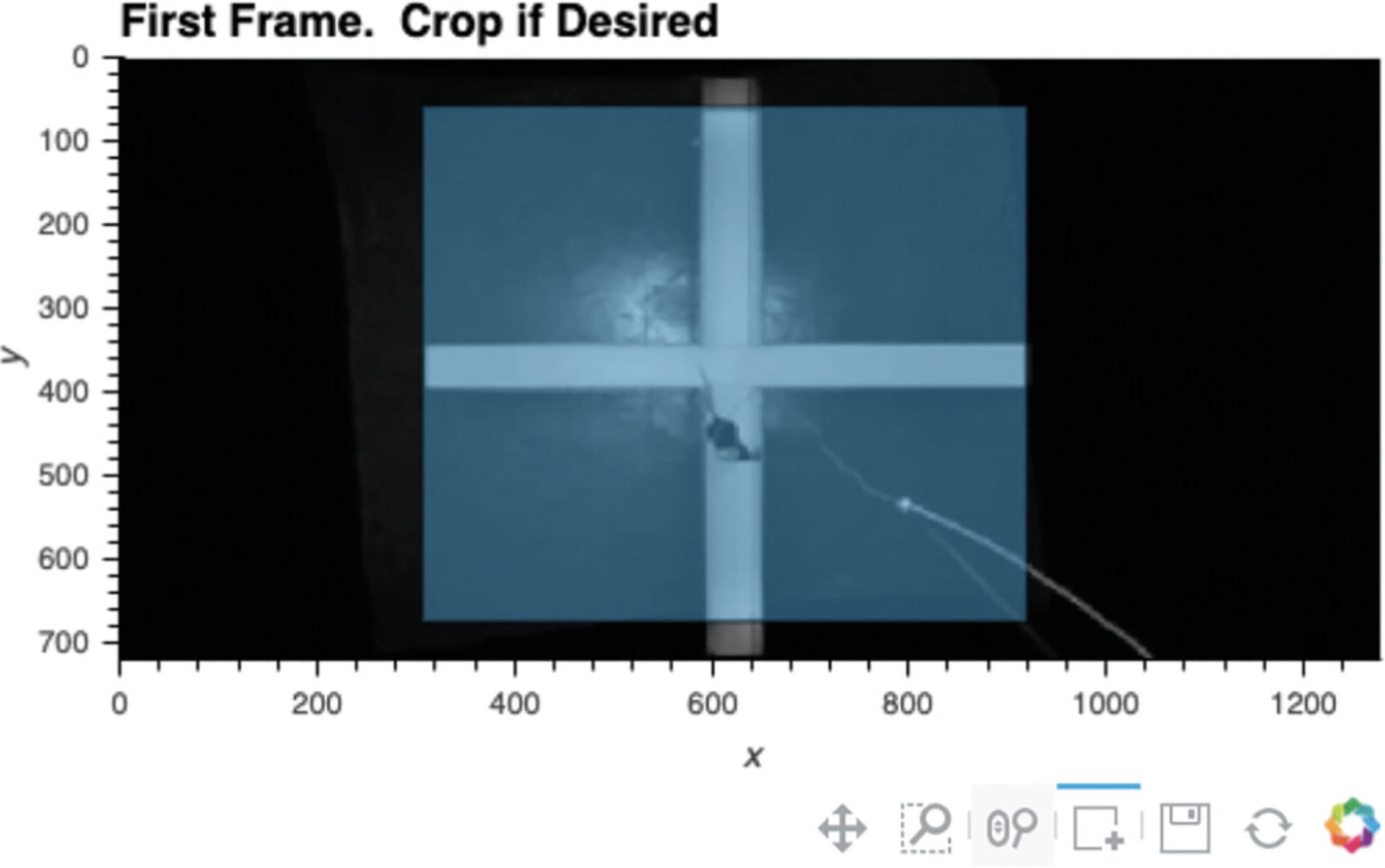
4.Mask regions (optional).
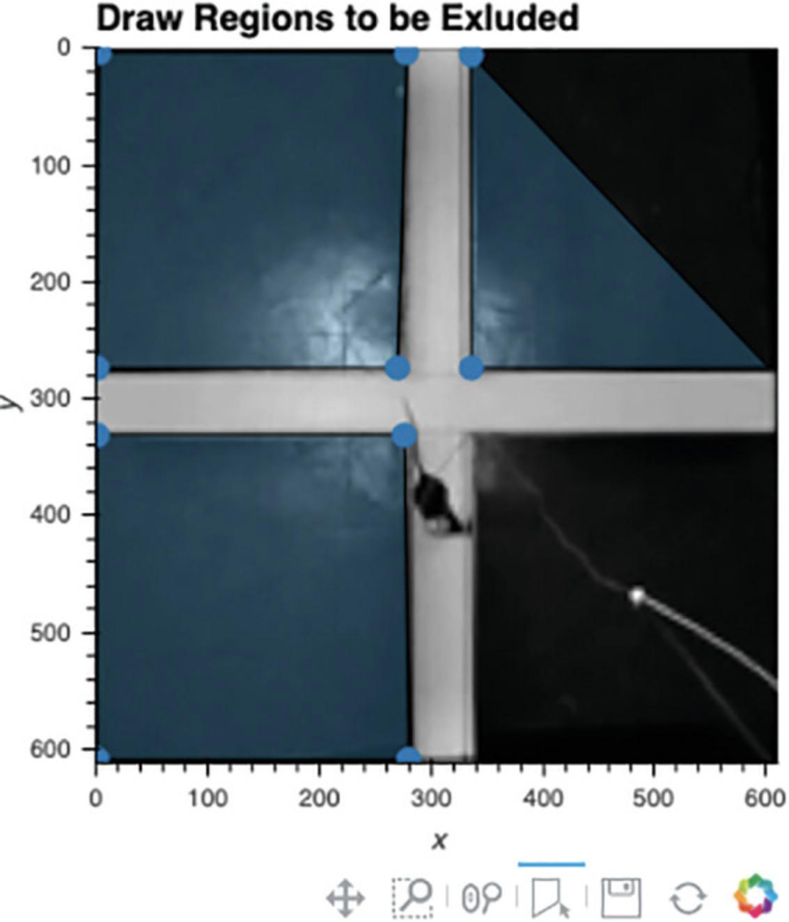
Cell 4 can be used to select one or more regions that the user would like ignored during processing (see Fig. 4). This can be helpful if there is movement in that portion of video due to the experimenter stepping into the field of view or other external movements. Any polygonal region can be drawn, and as many regions as desired can be masked. Because the selected regions will be ignored, be sure not to select any region that the tracked animal can enter into.
- a.Run Cell 4.The first frame of the video will appear, with any cropping from the prior cell applied.
- b.To draw a region to be ignored, double-click on the image to identify its first vertex, single-click to add each additional vertex, and double-click again to finalize each region.
5.Define the reference frame for location tracking.
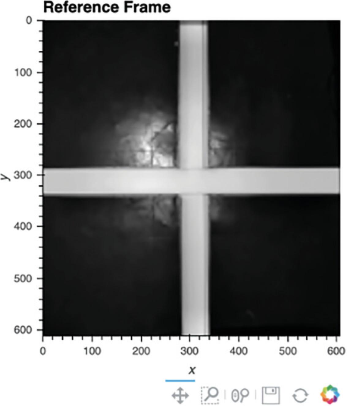
For location tracking to work, a view of the arena without an animal must be generated (Fig. 5). There are two ways to do this. Option 1 provides a method to remove the animal from the video. This works well provided that the animal does not stay in the same location for >50% of the session. Alternatively, Option 2 allows the user to define a video file, in the same folder as the video being scored, that does not have an animal in it. Option 1 is generally recommended because it is simpler for the user to acquire and ensures the reference frame is consistent with the video. If an alternative video is used, we recommend that the user acquire a short video (e.g., 5 s) of the empty arena on each experimental day.
- a.Option 1 : Create reference frame by removing animal from video.
Run the cell under Option 1.An image of the environment lacking an animal should appear (Fig. 5).
- b.Option 2 : Specify a video of the empty box (preferable only if the animal moves very little).
Run the cell under Option 2 after specifying the name of the alternative file within the cell. An image of the environment lacking an animal should appear (Fig. 5).
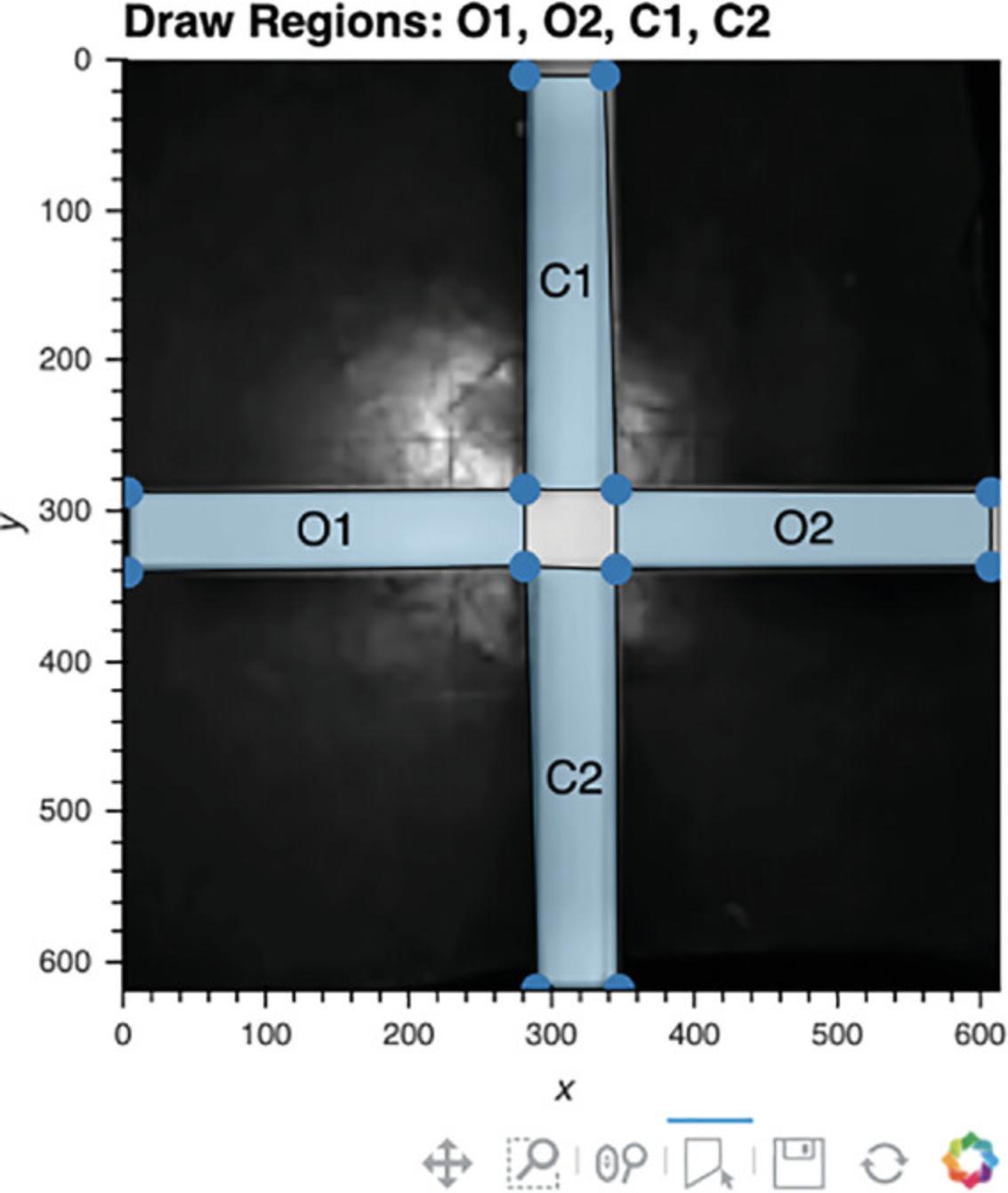
6.Use interactive plot to define regions of interest (optional).
-
Run Cell 6. The reference frame will appear (Fig.6).
-
The user can now draw the regions of interest in the order listed above the reference frame. To draw a region, double-click on the image to identify its first vertex, single-click to add each additional vertex, and then double-click again to close this region.
7.Define scale for distance calculations.
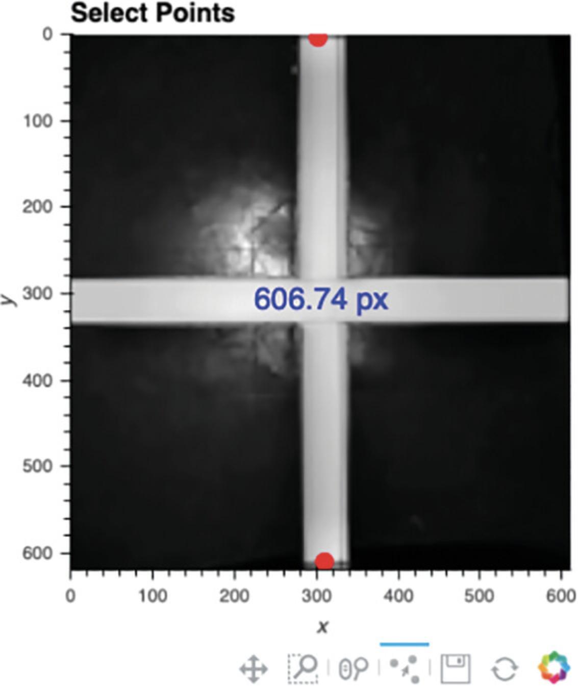
ezTrack initially tracks distance in pixel units. To convert from pixel units to a physical scale (inches, centimeters, etc.), the user can select any two points in the reference frame (Cell 7a), and then once supplied with their true physical distance (Cell 7b), ezTrack will provide distance measurements at the desired scale.
-
Select two points of known distance.iRun Cell 7a; the reference frame will appear.iiClick on any two points on the reference frame. The distance between them will be presented in pixel units (Fig.7).
-
Define the real-world distance between points.
Set the values of the variables “distance” and “scale” in Cell 7b; then run the cell. If the distance between the two selected points is 100 centimeters, the user would set the code as follows:
distance = 100
scale = ‘cm’
Note that “scale” will take any set of characters within quotations, so “centimeters” would have worked just as well as “cm.”
8.Track location.
Cells 8a-d are used to test and choose tracking parameters, and once selected, track the location of an animal across an entire video.
-
Set Location Tracking parameters.
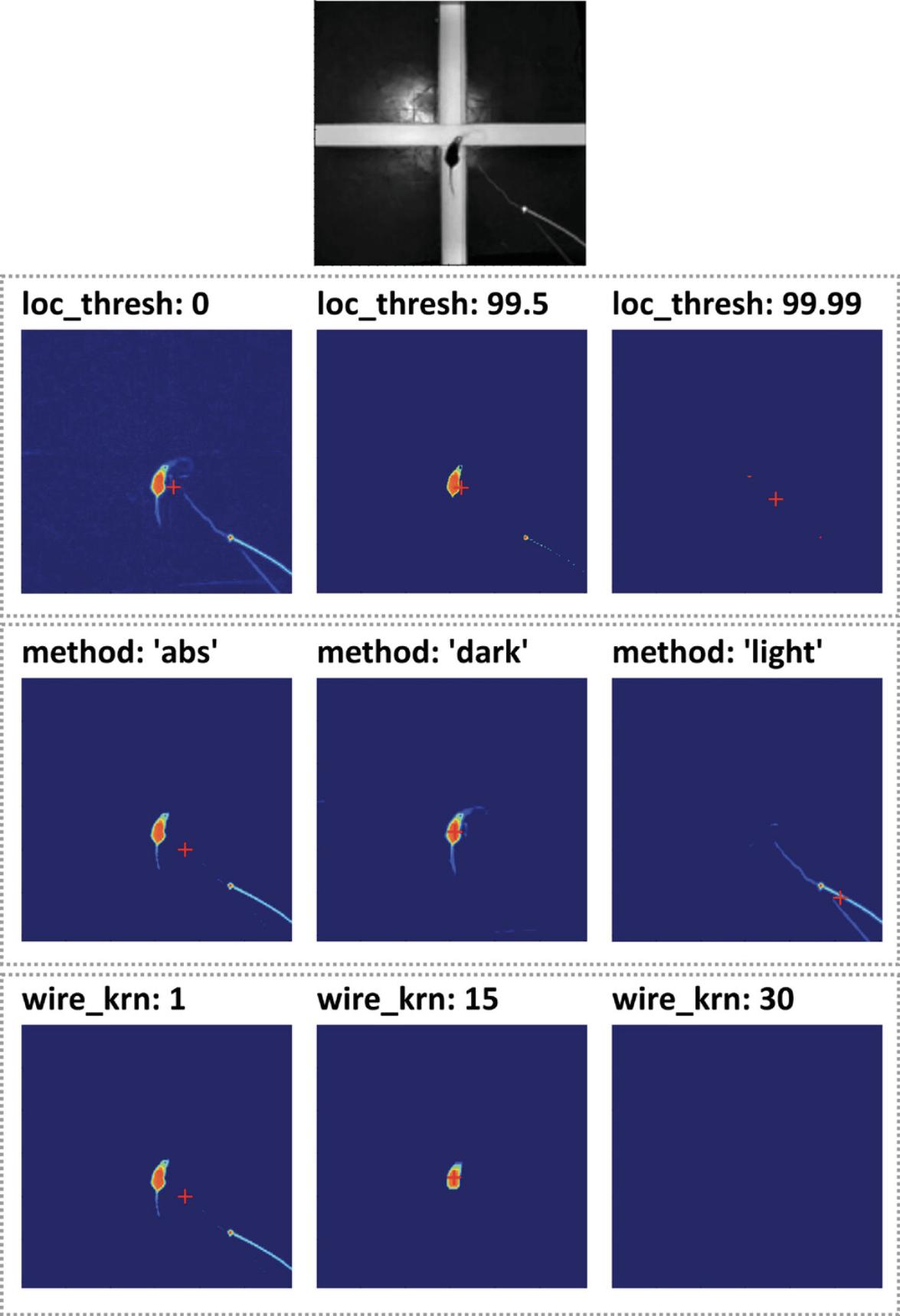
In Cell 8a, the user defines a number of tracking parameters (see Fig. 8), each of which is described below. The defaults will often work well. However, in Cell 8b, the user can quickly visualize the accuracy of tracking with these parameters on a subset of video frames and modify parameters as they see fit. The idea is to cycle between Cell 8a and Cell 8b until one is happy with the chosen tracking parameters, and then proceed to track the entire video. Each of these parameters is described below, and the influence of changing several parameters can be seen in Figure 9.
loc_thresh : The parameter loc_thresh represents a percentile threshold and can take on values between 0 and 100. Each frame is compared to the reference frame. Then, to remove the influence of small fluctuations, any differences below a given percentile (relative to the maximum difference) are set to 0. The impact of changing this parameter can be seen in Figure 9.
use_window : The parameter use_window is incredibly helpful if objects other than the animal temporarily enter the field of view during tracking (such as an experimenter's hand manually delivering a stimulus or reward). When use_window is set to True, a square window with the animal's position on the prior frame at its center is given more weight during searching for the animal's location (because an animal presumably cannot move far from one frame to the next). In this way, the influence of objects entering the field of view can be avoided. If use_window is set to True, the user should consider window_size and window_weight.
window_size : This parameter only affects tracking when use_window is set to True. This defines the size of the square window surrounding the animal that will be more heavily weighted in pixel units. We typically set this to two to three times the animal's size (if an animal is 100 pixels at its longest, we will set window_size to 200). Note that to determine the size of the animal in pixels, the user can reference any image of the arena presented in ezTrack, which has the pixel coordinate scale on its axes.
window_weight : This parameter affects tracking only when use_window is set to True. When window_weight is set to 1, pixels outside the window are not considered at all; at 0, they are given equal weight. Notably, setting a high value that is still not equal to 1 (e.g., 0.5-0.9) should allow ezTrack to more rapidly find the animal if, by chance, it moves out of the window.
method : The parameter method determines the luminosity of the object ezTrack will search for relative to the background and accepts values of “abs,” “light,” and “dark.” The option abs does not take into consideration whether the animal is lighter or darker than the background and will therefore track the animal across a wide range of backgrounds, whereas light assumes the animal is lighter than the background, and dark assumes the animal is darker than the background. Option abs generally works well, but there are situations in which you may wish to use the others. For example, if a tether is being used that is opposite in color to the animal (e.g., a white wire and a black mouse), the abs method is much more likely to be biased by the wire, whereas dark will look for the darker mouse (see the example in Fig. 9).
rmv_wire : When rmv_wire is set to True, an algorithm is used to attempt to remove wires from the field of view. If rmv_wire is set to True, the user should consider wire_krn.
wire_krn : This parameter only affects tracking when rmv_wire is set to True. This value should be set between the width of the wire and the width of the animal, in pixel units. As can be appreciated from Figure 9, when this value is too small, the influence of the wire is not mitigated at all. When the value is too large, the animal is removed from the video.
- b.Display examples of location tracking to confirm parameters (optional).
After selecting parameters in the previous step, the user can run Cell 8b to visualize the impact of these parameters on a small subset of frames (the default is four frames).
A random selection of frames is analyzed, and the frames are then presented, with the animal's position marked with a crosshair. Side by side with the original image, the user can also visualize the features of each frame that are being used by ezTrack to mark the location of the animal. See Figure 9 for examples of when tracking is done well and when it is done poorly.
Of note, because frames are processed individually, the impacts of use_window, window_size, and window_weight are not visible here, since the window weighting algorithm requires knowledge of the animal's position on the prior frame. The impacts of the window weighting algorithm are better observed in Cell 10, where a video of tracking can be played.
- c.Track location and save results to a .csv file.
By running Cell 8c, the entire video will be tracked. The resulting .csv file (the video filename with the suffix _LocationOutput) will contain the following information for each frame: the animal's x and y coordinates in pixel units, whether or not the animal is in each supplied region of interest (True/False, for each), and the distance the animal has traveled relative to its position on the previous frame in both pixel units and any other scale the user might have provided. The first five rows of this file will be presented in the notebook.
- d.Display animal distance/location across a session (optional).
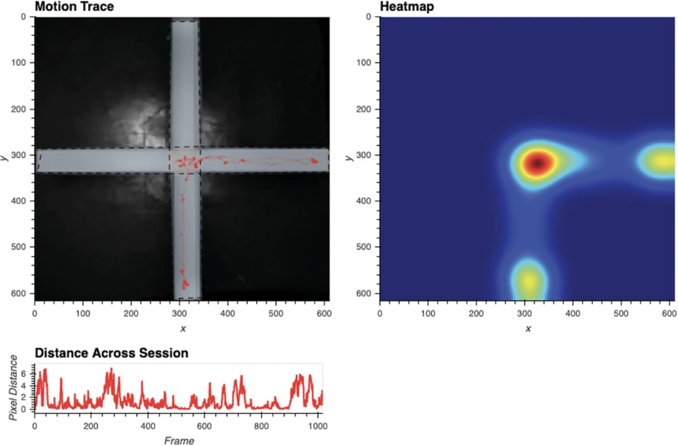
Run Cell 8d to acquire several visualizations of the performed tracking (Fig. 10). This includes a plot titled “Motion Trace,” which displays the animal's position on every frame atop the reference frame. This is useful in identifying whether any external movement has biased tracking. For instance, one would not expect the animal to ever be located outside of the arena. A plot titled “Heatmap” is also presented, which allows the user to visualize the relative amount of time the animal has spent in each area of the arena. Lastly, the plot “Distance Across Session” shows how much the animal moves on a frame by frame basis. This plot is particularly useful for detecting poor tracking, often evident in sudden leaps in distance traveled. The exact distance of such a leap will depend upon the video, but will likely be several standard deviations above the rest of the video. When such deviations are seen, it is useful to play video of the affected frames in Cell 10 to determine the source of the error.

9.Create binned summary report and save (optional).
In Cell 9, the user is able to obtain summary information, either for defined time bins or the entire tracking period. For each time bin requested, the total distance traveled and the proportion of time in any defined regions of interest will be saved to a .csv file (a file with the video filename with the suffix _SummaryStats). Refer to Figure 11 for an example of how to define bins. The name of each bin should be placed in quotation marks, while the numbers inside the parenthesis are the frames you want the bin to begin and end with. A comma should separate each bin. Note that defined frames are relative to the defined start frame (from Cell 2), such that 0 refers to the first tracked frame. If the user wants a summary of the entire tracking period, set bin_dict equal to None. In addition, if it's easier for the user to think in seconds, as opposed to frames, multiplication can be done within the parenthesis. For example, assuming a frame rate of 30, the following would create bins for seconds 0-100, 100-200, and 200-300:
bin_dict = {
ˈBinName1ˈ: (030, 10030),
ˈBinName2ˈ: (10030, 20030),
ˈBinName3ˈ: (20030, 30030)
}

10.View video of tracking.
After tracking has been performed, Cell 10 allows the user to play a portion of the video back with the animal's position marked on each frame with a crosshair. After defining the display parameters by setting the values of display_dict, running Cell 10 will result in the video being played (see Fig. 12). Below we outline the meaning of each of these parameters.
start : The frame video playback is to be started on. Note that this is relative to the start of tracking, where 0 is the first tracked frame (the defined start frame from Cell 2)
stop : The frame video playback is to end on. Note that this is relative to the start of tracking, where 0 is the first tracked frame (the defined start frame from Cell 2)
fps : The speed of video playback. Must be an integer. Video playback may also be slower depending upon computer speed. This is because “fps” sets the time imposed between presented frames but cannot control the duration of time it will take a user's computer to present each frame.
resize : If the user wants the output to be larger or smaller, or they want the aspect ratio to be different, resize can be supplied as in the following example:
ˈresizeˈ: (100,200)
Here, the first number corresponds to the adjusted width of the frame, whereas the second number corresponds to the adjusted height. Both numbers reflect pixel units and should be integers. Set resize equal to None if no resizing is to be done.
save_video: To save the video clip, set “save_video” to True.

Process multiple files in a batch (LocationTracking_BatchProcess.ipynb)
Batch processing with ezTrack works much the same way as individual processing but is designed to be executed on all video files of a specified type within a given folder. The user will find that many of the steps are identical to individual processing, with the following exceptions. First, rather than specifying the directory and the name of an individual file, the user supplies the directory and the file extension of the videos to be processed. ezTrack will process all files of the specified file type within the given folder. Second, when batch processing, all cropping parameters, bin information, and regions of interest are assumed to be the same. The user should therefore be mindful that videos should have a consistent field of view and be of a roughly similar length. Third, the user is still able to crop the videos, supply regions of interest, mask portions of the field of view, and supply distance scales—however, these are based upon the first video file in the folder. Again, be mindful to ensure that videos are roughly the same, although minor discrepancies in the field of view are permissible. Fourth, the batch processing notebook file does not contain visualization tools to optimize tracking parameters, as it is assumed that these have been previously explored while processing a few individual files. However, at the end of processing, heatmaps and motion trace plots for each video are displayed.
Basic Protocol 3: USING THE FREEZE ANALYSIS MODULE
ezTrack's Freeze Analysis Module assesses an animal's motion and freezing across the course of a single, continuous session. The Freeze Analysis Module tracks the number of pixels that fluctuate from one frame to the next and uses this as an index of animal motion. This metric arguably provides greater sensitivity than measuring the animal's center of mass, as is done in the Location Tracking Module, while sacrificing information regarding animal position. Subsequently, the user defines a threshold for motion (both in magnitude and duration) below which freezing is defined. In this way, motion is converted into a binary variable, freezing. The Freeze Analysis Module saves frame by frame motion/freezing data in convenient and accessible .csv files. Summary files can also be created specifying the average motion and freezing in user-defined time bins. The Freeze Analysis Module can be used to process an individual video file or several video files in batch.
Below, we first describe the protocol for video calibration (using FreezeAnalysis_Calibration.ipynb), which allows the user to better separate pixel fluctuations that result from animal movement from those due to stochastic fluctuations inherent in video acquisition. For this reason, if the user would like to utilize calibration, it is important to record a video of the empty arena before starting behavioral recording. A single 5- to 10-s video is typically sufficient. Next we outline the protocol for utilizing the Freeze Analysis Module to analyze a single video, FreezeAnalysis_Individual.ipynb. This protocol provides the user with an array of visualization tools to explore parameter settings in order to confirm accurate measurement of freezing. We highly recommend using this protocol on a few individual videos from each experiment before proceeding to process multiple videos in batch. Lastly, given the large degree of overlap between processing individual files and batch processing, we briefly discuss batch processing (FreezeAnalysis_BatchProcess.ipynb), with differences from individual processing highlighted.
Necessary Resources
Please see Strategic Planning regarding hardware/software considerations
Open the relevant Freeze Analysis file
i. Activate the ezTrack environment.
For OSX/Linux users, open a terminal. If using Windows, open Anaconda Prompt. Type the following command and then hit Enter:
conda activate ezTrack
ii. Launch Jupyter Notebook.
Within Anaconda Prompt/Terminal, type the following command and then hit Enter:
jupyter notebook
iii. Select Notebook file from Jupyter Notebook.
Within Jupyter Notebook, navigate to the folder containing the ezTrack files downloaded from the Github site, and open either FreezeAnalysis_Calibration.ipynb, FreezeAnalysis_Individual.ipynb, or FreezeAnalysis_BatchProcess.ipynb.
Calibration
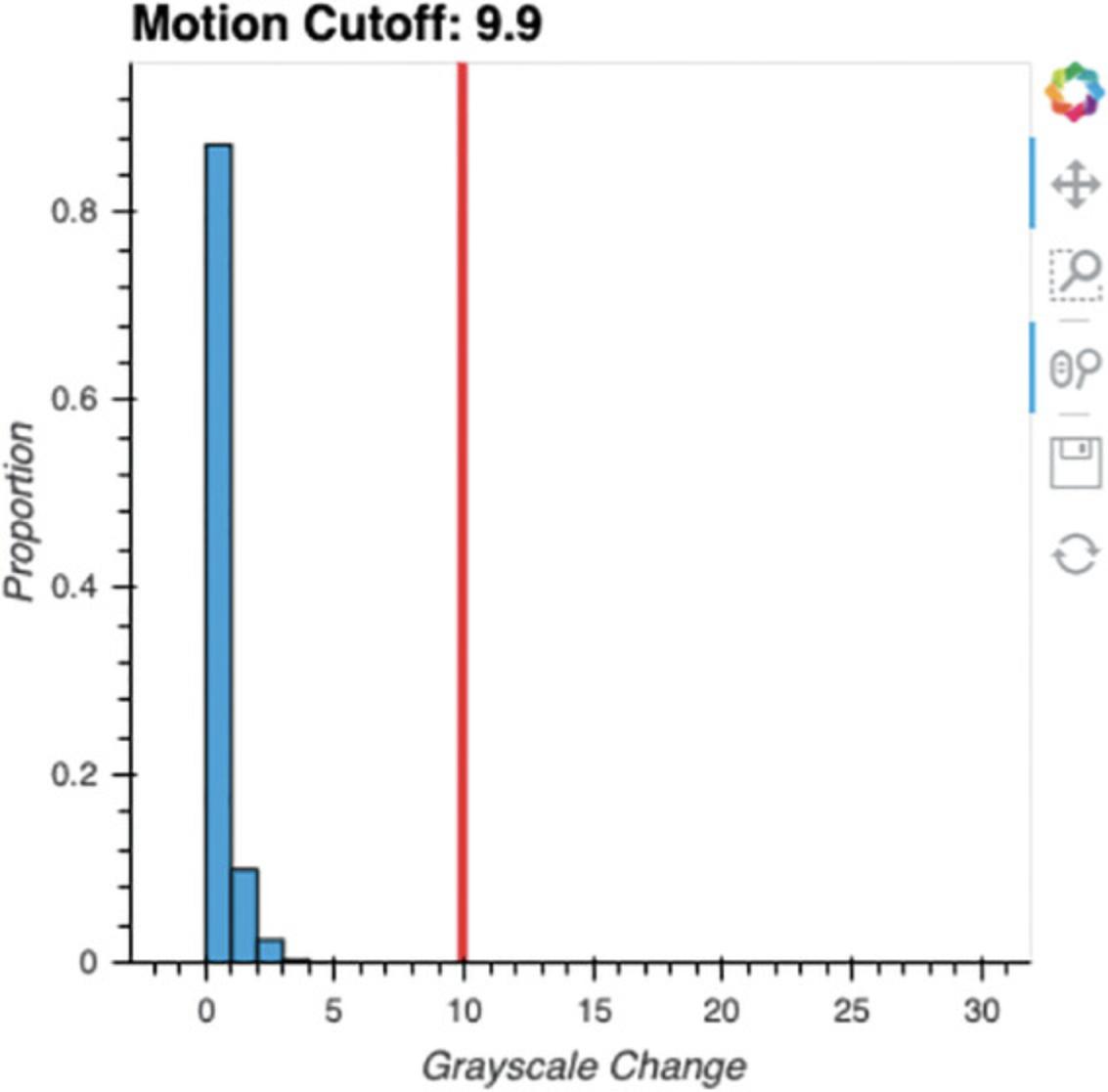
Even when there is no movement in the field of view, pixel brightness values fluctuate slightly from frame to frame. As such, values would be greatly biased if any pixel fluctuation was counted as animal motion. By determining the magnitude and distribution of these random fluctuations when no animal is present, one can more easily define pixel fluctuations that are actually due to the movement of an animal. Provided that the user has a short video of their environment without an animal (e.g., 5-10 sec), the user can visualize this distribution and use this to select a cutoff for subsequent steps.
Note that the numbering of the following instructions corresponds to the numbered blocks of code in the Jupyter Notebook file (called “cells”). Some of these cells are optional, as noted both here and in the Jupyter Notebook file itself.
1.Load necessary packages.
Running Cell 1 loads all necessary packages and does not need to be modified.
2.Set directory and file information.
In Cell 2, the user specifies the video file location and other pertinent information about the video, described below (see Fig. 13). After entering this information, run the cell.
dpath : The directory path of the folder containing the video to be processed.
file : The filename of the video, including the file extension.
cal_frms : The number of frames in the video to calibrate based upon. If the video is 10 sec long and was shot at 30 frames/sec, the user might set this to 300. If the user is unsure of the frame rate, this information will be output by ezTrack when Cell 3 is run. Note that for longer videos, it is not necessary to calibrate based upon the total number of frames in the video.
dsmpl : The amount to down-sample each frame. If processing is going slowly, down-sampling can help. A value of 1 indicates no down-sampling, while a value of 0.25 indicates that the frame will be down-sampled to one-quarter the original size. Note that if the user chooses to down-sample in the calibration step, this same down-sampling factor should be used for processing behavioral videos, and vice versa.
stretch : Allows the user to alter the aspect ratio of the presented output. This is useful when videos have irregular dimensions and are difficult to see (e.g., an aspect ratio of 1:100). The width/height will be scaled by the factor provided. Note that this only affects the appearance of visualizations and does not modify the video or the interpretation of the output.

3.Load video information. Display first frame.
Run Cell 3 to load the video. The starting frame of the video will appear as output, and various video properties will also be printed, including the filename, the number of frames in the video, the frame rate, and the frame dimensions. If you would like to alter the size of the image output, the number in the first line of this cell (i.e., %% output size = 100) can be increased or decreased accordingly. If the dimensions of your video frame are very small, sometimes no image will appear. Increasing the output size to 200 or more will remedy this. If a “FileNotFoundError” emerges, the user should double-check that directory path and filename are correctly specified.
4.Calibrate video.
When Cell 4 is run, ezTrack examines how pixel grayscale intensities change on a frame-by-frame basis across the specified length of the video. A histogram displaying these grayscale intensity changes is output (Fig. 14). By looking at the distribution of frame-by-frame change values, a threshold can then be set for determining what changes are likely to be attributable to an animal moving versus random fluctuation. This threshold is subsequently used when analyzing videos with animals in them. Currently, a suggested cutoff is printed corresponding to twice the 99.99th percentile. However, the user can adjust this value to suit their needs. Zooming tools adjacent to the plot can be used to more closely examine low-frequency change values.
Process an individual file (FreezeAnalysis_Individual.ipynb)
Note that the numbering of the following instructions corresponds to the numbered blocks of code in the Jupyter Notebook file (called “cells”). Some of these cells are optional, as noted both here and in the Jupyter Notebook file itself.
1.Load necessary packages.
Running Cell 1 loads all necessary packages and does not need to be modified.
2.Set directory and file information.
In Cell 2, the user specifies the file's location and other pertinent information about the video, described below (see Fig. 15). After entering this information, run the cell.
dpath : The directory path of the folder containing the video to be processed. Note that if you are using a Windows path with backslashes, place an “r” in front of the directory path to avoid an error (e.g., r’\Users\DeniseCaiLab\Videos’).
file : The filename of the video, including the file extension.
start : The frame of the video on which to begin processing. 0 is the first frame. By knowing the video's frame rate (e.g., 30 frames/sec), the user can start processing the video at a specific timepoint. For instance, to begin processing 20 sec into the video, once the animal has been placed into the arena, one could enter 600 if the frame rate were 30 frames/sec. If you are uncertain of your video's frame rate, this information will be printed by ezTrack when Cell 3 is run.
end : The frame of the video to end processing on. If the user would like to process from the start frame to the end of the video, this can be set to None.
dsmpl : The amount to down-sample each frame. If processing is going slow, down-sampling can help. A value of 1 indicates no down-sampling, while a value of 0.25 indicates that the frame will be down-sampled to one-quarter the original size. Note that if down-sampling is performed, all pixel coordinate output will be in the dimensions of the down-sampled video.
stretch : Allows the user to alter the aspect ratio of the presented output. This is useful when videos have irregular dimensions and are difficult to see (e.g., an aspect ratio of 1:100). The width/height will be scaled by the factor provided. Note that this only affects the appearance of visualizations and does not modify the video or the interpretation of the output.

3.Load video, and crop frame if desired.
-
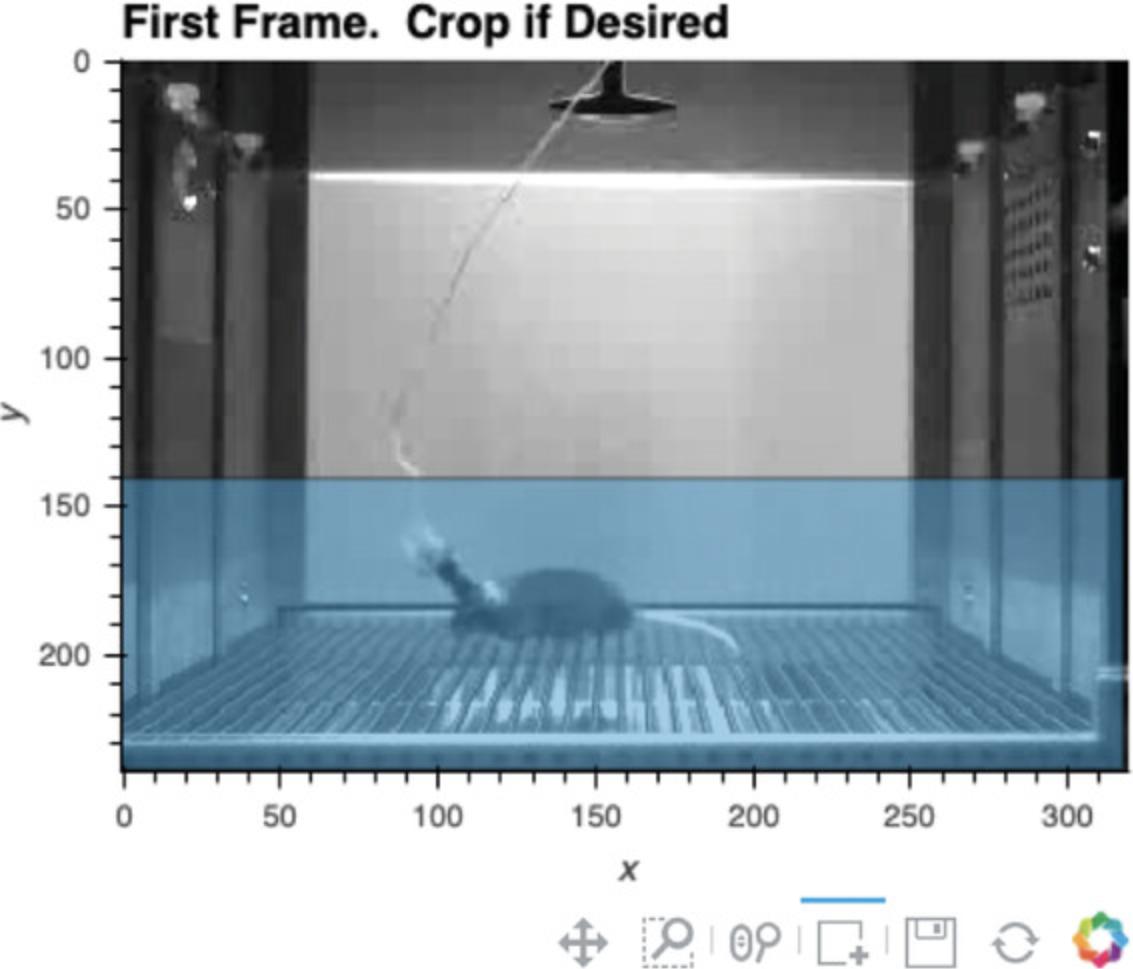
Run Cell 3 to load the video. The video's starting frame will appear as output, and various video properties will also be printed, including the filename, the number of frames in the video, the frame rate, and the frame dimensions.
-
The user can then define how to crop the video at this stage, if desired (see Fig.16). Select the box selection tool below the presented image (the square with a plus sign) and double-click the image to begin defining the region you would like your video cropped to. Double-click again to finalize the region. If the region is not satisfactory, rerun Cell 3 and follow the steps for cropping again.
If you would like to alter the size of the image output, the number in the first line of Cell 3 (i.e.,%% output size = 100) can be increased or decreased accordingly. If the dimensions of the video frame are very small in one dimension (such as on a long linear track), sometimes no image will appear. Increasing the output size to 200 or more will remedy this. If a “FileNotFoundError” emerges, the user should double-check that the directory path and filename are correctly specified.
4.Analyze motion across session.
In Cells 4a and 4b, the user defines a threshold for detecting frame-by-frame pixel fluctuations that are indicative of motion, and ezTrack then calculates motion across the session.
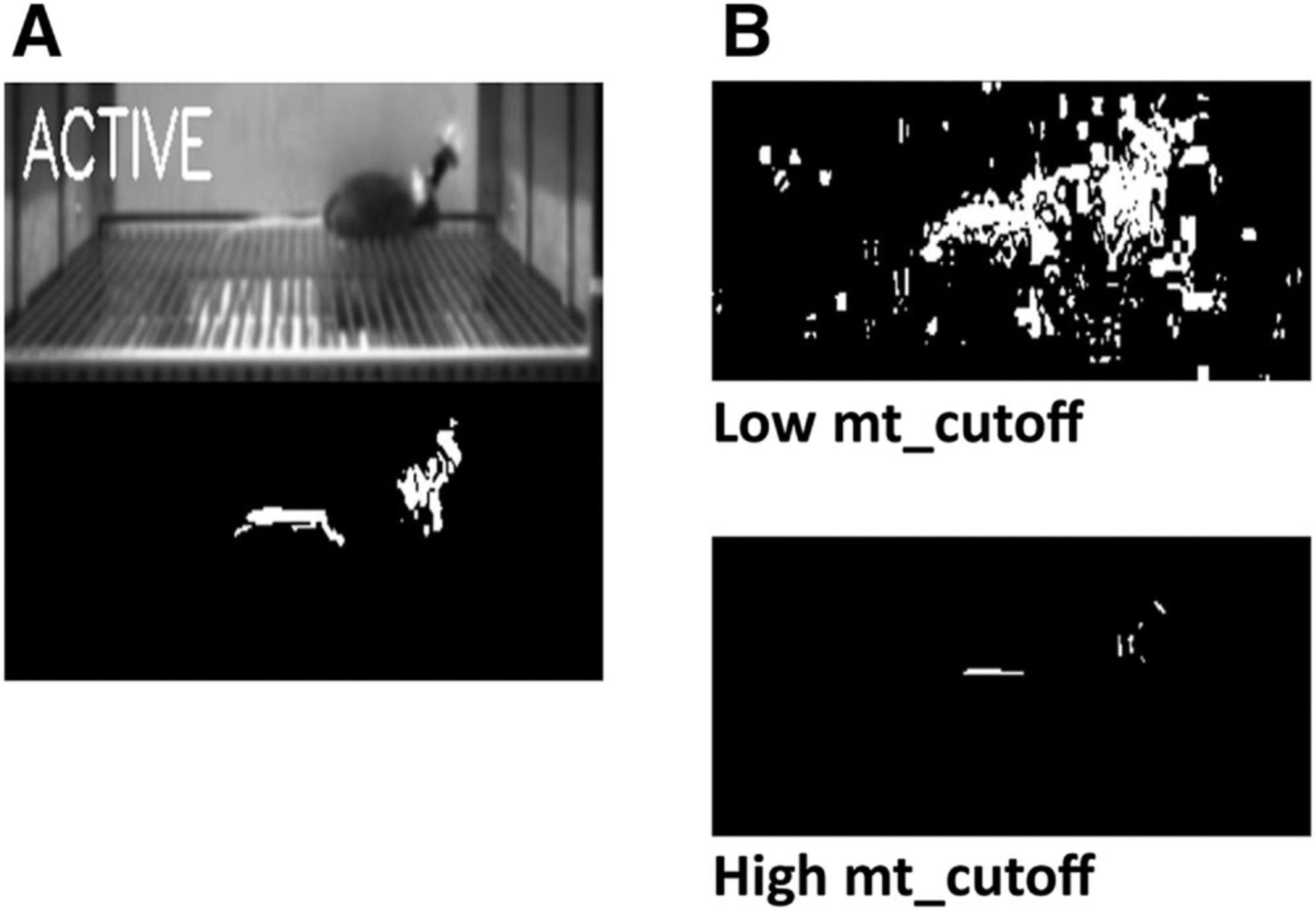
- Set motion threshold. To measure motion, ezTrack's Freeze Analysis Module detects the number of pixels that change in intensity from one frame to the next. However, a certain degree of variability is expected by chance and not due to the motion of the animal. To account for this, the user must set a threshold, “mt_cutoff,” defining how large a pixel intensity change is enough to count as motion. Define this threshold in Cell 4a and run the cell.
Using too small a cutoff will result in motion being detected even when the animal is motionless; too high a cutoff will result in no motion being detected when the animal is moving. If the user has run the Calibration protocol,mt_cutoffcan be set to the suggested value. The impact of this parameter can be visualized in Cell 6. Again, see steps 4-7 for a protocol to estimate a good cutoff.
-
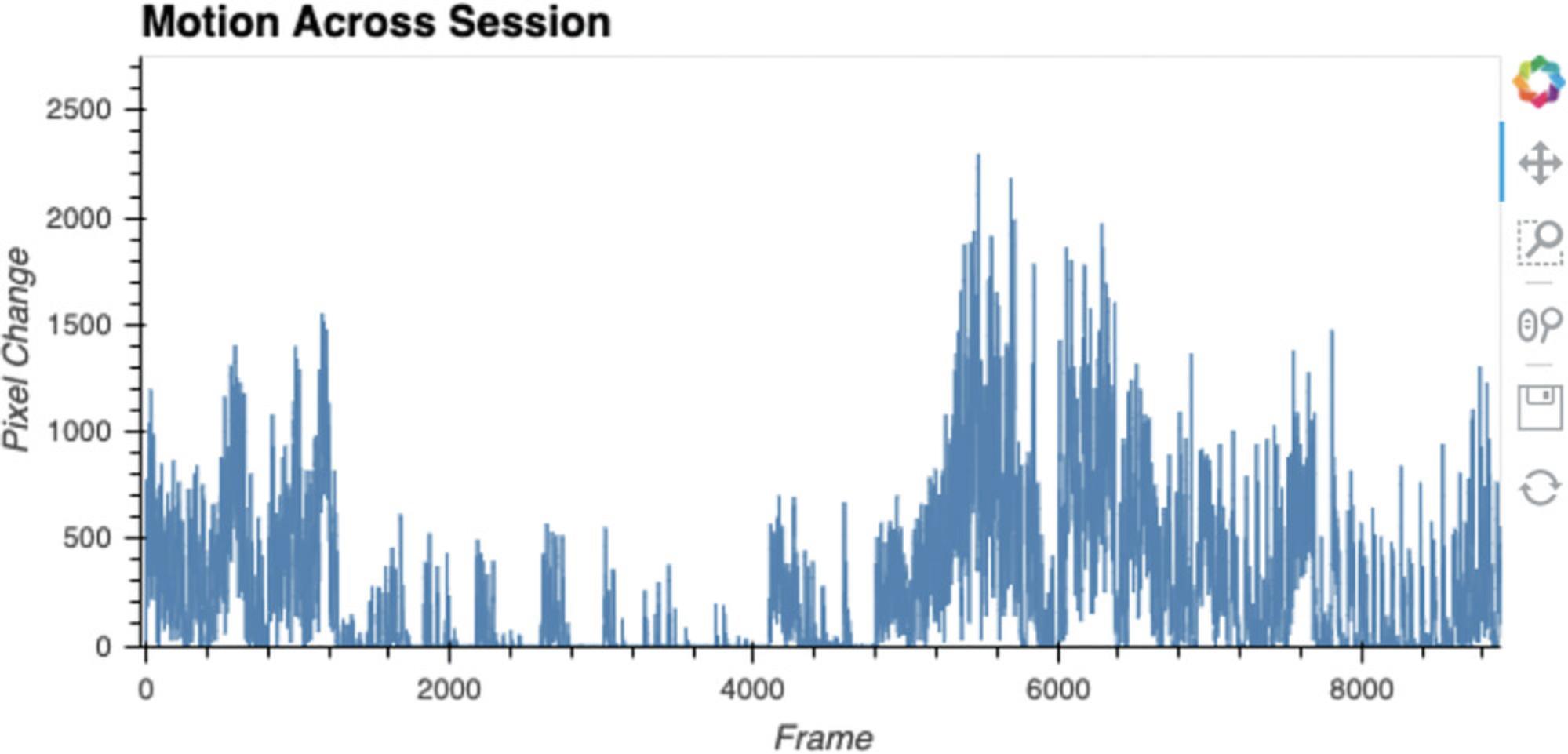
Detect motion and plot. Run Cell 4b. Here, ezTrack loops through all frames and detects the number of pixels whose grayscale change exceedsmt_cutoffper frame. The results are then plotted in an interactive nature. In addition to changing the overall output size in the first line of this cell, the aspect ratio can also be changed. In line 3 of this cell, the height (h) and width (w) of the plot are chosen as follows:
h, w = 300, 1000
The first number reflects the height of the plot, and the second number reflects the width.
5.Analyze session freezing.
In Cells 5a and 5b, the user first defines the maximal amount of motion the animal can exhibit and be considered to be freezing (FreezeThresh), as well as the duration the animal must remain below this cutoff (MinDuration) to be considered freezing.
-
Select freezing parameters.
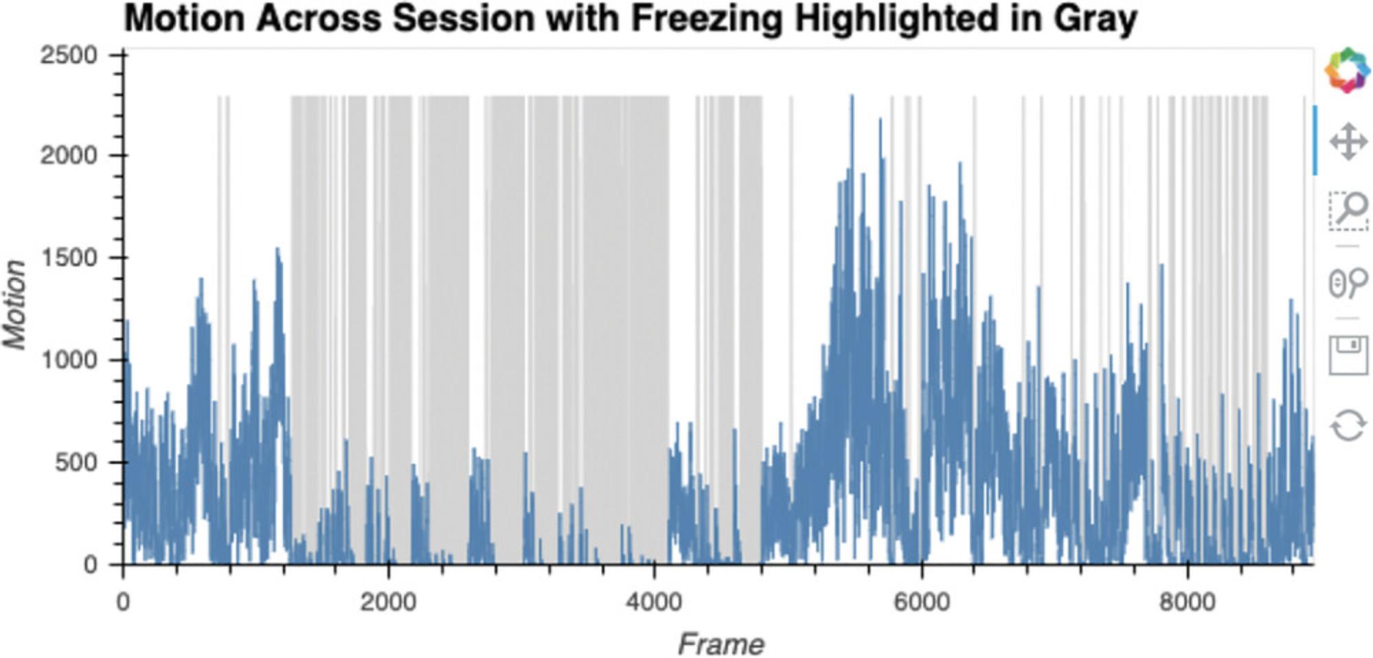
Here, the user sets FreezeThresh, corresponding to the maximal number of pixels per frame that can change (i.e., motion) where the animal would still considered to be freezing. This can first be set by examining motion values in the output to Cell 4b (Fig. 17). A value should be chosen that captures the low troughs in motion, likely attributable to freezing, and should not be so low that very small blips (attributable to breathing or slight head bobbing) in motion are counted. In Figure 17, for example, a value between 100 and 200 would likely be appropriate. However, this can be subsequently titrated to user preference by watching video playback in Cell 6.MinDuration reflects the duration, in frames, that the animal's motion must drop below FreezeThresh before freezing accrues. This is often set in the 0.5- to 1-sec range.
- b.Measure freezing and save.
Here, ezTrack determines freezing on a frame-by-frame basis and saves the data (Figure 18). The resulting .csv file (the video filename with the suffix _FreezingOutput, in the folder containing the video file) will contain the following information for each frame: the amount of motion (in pixel change units) and whether or not the animal is freezing (0 = not freezing, 100 = freezing). The results are then plotted in an interactive nature. The dimensions of this plot can be changed in the same way described for Cell 4b.
6.Play video with scoring.
After scoring has been performed, Cell 6 allows the user to play back a portion of the video (Fig. 19). Classification of the animal as active/freezing is displayed (Fig. 19). Additionally, the detected motion in the video is made visible. After the display parameters have been defined by setting the values of display_dict, running Cell 6 will result in the video being played. Below we outline the meaning of each of these parameters (Fig. 20).
start : The frame video playback is to be started on. Note that this is relative to the start of tracking, where 0 is the first tracked frame (the defined start frame from Cell 2).
stop : The frame video playback is to end on. Note that this is relative to the start of tracking, where 0 is the first tracked frame (the defined start frame from Cell 2).
fps : The speed of video playback. Must be an integer. Video playback may also be slower depending upon computer speed. This is because fps sets the time imposed between presented frames but cannot control the duration of time it will take a user's computer to present each frame.
resize : If the user wants the output to be larger or smaller, or the aspect ratio to be different, resize can be supplied as in the following example:
‘resize’: (100,200)
Here, the first number corresponds to the adjusted width of the frame, whereas the second number corresponds to the adjusted height. Both numbers reflect pixel units and should be integers. Set resize equal to None if no resizing is to be done.
save_video: If the user would like to save the video clip, save_video can be set to True.

7.Create binned summary report and save (optional).
In Cell 7, the user is able to obtain summary information, either for defined time bins or the entire tracking period. For each time bin requested, the animal's average motion and freezing will be saved to a .csv file (a file with the video filename with the suffix “_SummaryStats” in the folder containing the video file). Refer to Figure 21 for an example of how to define bins. Each bin's name should be placed in quotation marks, while the numbers inside the parenthesis indicate the bin's desired start and end frames. Each bin should be separated by a comma. Note that defined frames are relative to the defined start frame (from Cell 2), such that 0 refers to the first tracked frame. If the user wants a summary of the entire tracking period, set bin_dict equal to None. In addition, if it is easier for the user to think in seconds, as opposed to frames, multiplication can be done within the parenthesis. For example, assuming a frame rate of 30, the following would create bins for seconds 0-100, 100-200, and 200-300:
bin_dict = {
ˈBinName1ˈ: (030, 10030),
ˈBinName2ˈ: (10030, 20030),
ˈBinName3ˈ: (20030, 30030)
}

Process multiple files in a batch (FreezeAnalysis_BatchProcess.ipynb)
Batch processing with ezTrack works much the same way as individual processing, but is designed to be executed on all video files of a specified type within a given folder. The user will find that many of the steps are identical to individual processing, with the following exceptions. First, rather than specifying the directory and the name of an individual file, the user supplies the directory and the file extension of the videos to be processed. ezTrack will process all files of the specified file type within the given folder. Second, when batch processing, all cropping parameters and bin information are assumed to be the same. The user should therefore be mindful that videos have a consistent field of view and be of a roughly similar length. Third, the user is still able to crop the video, as with individual processing; however, cropping is based upon the first video file in the folder. Again, be mindful that videos need be roughly the same, although minor discrepancies in the field of view are permissible. Fourth, the batch processing notebook file does not contain visualization tools to optimize tracking parameters. It is assumed that these have been previously explored while processing a few individual files.
COMMENTARY
Background
The measurement of animal behavior in the lab is commonplace across bioscience disciplines. It is therefore incredibly unfortunate that commercial resources for this task often cost several thousand dollars. This is a significant barrier to many scientific groups, including early-career investigators who have yet to obtain substantial funding, investigators from under-represented groups that have been historically underfunded, and research groups outside of large-scale institutions in the United States. Even for well-funded labs, justifying investing in costly equipment for short-term experiments can be difficult. Being entirely free and with no operating system or hardware requirements, we hope that ezTrack will help break down this barrier. We are thrilled that investigators around the world have already adopted ezTrack (https://github.com/DeniseCaiLab/ezTrack).
ezTrack is not the only free and open-source behavior tracking software. Other popular and attractive alternatives include DeepLabCut (Mathis et al., 2018), Bonsai (Lopes et al., 2015), MouseMove (Samson et al., 2015), Rodent Arena Tracker (Krynitsky et al., 2020), as well as many other great resources highlighted on the OpenBehavior website (edspace.american.edu/openbehavior). These software packages are fantastic and can sometimes offer distinct advantages over ezTrack, particularly when it comes to addressing ezTrack's limitations. For example, we recommend the use of DeepLabCut for detecting more nuanced behaviors, as well as for the measurement of multiple animals in the same arena. However, for the simpler behaviors ezTrack is set up to measure (see Table 1), ezTrack is likely faster to get running, requires less computing knowledge, and requires fewer computer resources (e.g., ezTrack does not entail GPU usage). Bonsai is another excellent option for real-time tracking and output control, being dedicated to acquiring input from multiple recording devices and controlling output devices, and provides relatively simple ways to set up sophisticated real-time workflows. However, setting up behavior tracking with Bonsai is less streamlined, if this is one's sole goal.
A major strength of ezTrack, relative to other commercial and open-source tracking options, is its breadth of functionality and the ease with which these features are implemented. Although other softwares are capable of implementing many of ezTrack's functions (see Table 1 for a review of ezTrack's capabilities), these options are not necessarily built into the workflow in a way that is readily apparent to the user. With ezTrack, each of these options is explicitly integrated into the ezTrack notebook files, making them more readily implemented. Our central goal has been to create a versatile and easy to use system for behavior measurement—developed by and made for behavioral scientists.
New features for ezTrack are continually under development, and we encourage users to follow ezTrack on Github to stay up to date. Since the original publication of ezTrack only a short time ago (Pennington et al., 2019), the ability to mask regions from the field of view, down-sampling, wire removal algorithms, and progress bars have all been added. Currently under development are resources to track behavior from webcams in real time to permit integration with output control devices, as well as methods to make it possible to track an animal's orientation along with their position. We hope these features will be available in the near future, and we look forward to working with the community to refine them.
Troubleshooting and Critical Parameters
We have attempted to discuss all critical parameters as well as possible issues that may arise in the preceding sections. As a final note, however, we highlight the major classes of issues one may encounter and outline a general framework for addressing them.
Tracking issues
If tracking does not achieve the desired accuracy, we first direct the user to review guidance on parameter selection within the relevant portion of the Basic Protocols, and the methods provided for visualizing the impact of changing each tracking parameter. We encourage using these parameter selection tools for each new experiment on a few representative videos before launching into batch processing. Even when the same recording environment is used across experiments, a change in camera settings, camera position, or room lighting may influence optimal parameter choice. For Location Tracking, Figure 9 can be particularly helpful regarding parameter selection guidance. For the Freeze Analysis Module, Figure 20 can be similarly helpful.
If altering parameters does not improve tracking, we encourage the user to review the capabilities and limitations of ezTrack in Strategic Planning and Table 1. The user should confirm that ezTrack can do what they would like it to. Lastly, we recommend the user review the section of Strategic Planning entitled General Considerations for Recording Behavior to assess if the way that their videos were acquired may have introduced problems into tracking.
Syntax issues
As with all programming languages, syntax must be relatively precise when changing code in ezTrack. Although minimal code is contained within the Jupyter Notebook files that the user interacts with, the user must still be mindful of the location of brackets, commas, quotation marks, etc. If any error messages emerge during use, this is often the first thing to check. It can be helpful to save a copy of the default files for comparison, in addition to examining example code in this manuscript (e.g., Figs. 2, 8, and 15).
Video incompatibility
Occasionally, a video file format may be encountered that is not supported by ezTrack. Fortunately, there are a host of free video converters available online that can be used to convert to formats that will be accepted by ezTrack (e.g., .avi with MPEG-4 codec).
Software bugs
Users occasionally encounter software bugs that must be fixed. For any errors encountered with ezTrack, issue reports can be submitted at https://github.com/DeniseCaiLab/ezTrack/issues.
Acknowledgments
This work was supported by the McKnight Memory and Cognitive Disorders Award to DJC, the Klingenstein-Simons Fellowship to DJC, the Brain Research Foundation Award to DJC, NARSAD Young Investigator Award to DJC, the Friedman Scholar Award to DJC, the One Mind Otsuka Rising Star Award to DJC, the Mount Sinai Distinguished Scholar Award to DJC, the Irma T. Hirschl/Monique Weill-Caulier Research Award to DJC, NIMH DP2MH122399-01 to DJC, NIMH R01MH120162 to DJC, the CURE Taking Flight Award to TS, the American Epilepsy Society Junior Investigator Award to TS, R03 NS111493 to TS, R21 DA049568 to TS, R01 NS116357 to TS, and NIDA 5T32DA007135 to ZTP.
Author Contributions
Zachary T. Pennington : Conceptualization, data curation, formal analysis, funding acquisition, investigation, methodology, project administration, resources, software, supervision, validation, visualization, writing-original draft, writing-review and editing; Keziah S. Diego : validation, writing-original draft, writing-review and editing; Taylor R. Francisco : validation, writing-original draft, writing-review and editing; Alexa R. LaBanca : validation, writing-original draft, writing-review and editing; Sophia I. Lamsifer : validation, writing-original draft, writing-review and editing; Olga Liobimova : validation, writing-original draft, writing-review and editing; Tristan Shuman : validation, writing-original draft, writing-review and editing; Denise J. Cai : conceptualization, data curation, formal analysis, funding acquisition, investigation, methodology, project administration, resources, software, supervision, validation, visualization, writing-original draft, writing-review and editing.
Conflict of Interest
The authors declare no conflict of interest.
Open Research
Data Availability Statement
All code for ezTrack can be found at https://github.com/DeniseCaiLab/ezTrack and is licensed under GNU GPLv3.
Literature Cited
- Bitzenhofer, S. H., Pöpplau, J. A., Chini, M., Marquardt, A., & Hanganu-Opatz, I. L. (2021). A transient developmental increase in prefrontal activity alters network maturation and causes cognitive dysfunction in adult mice. Neuron , 109, 1350–1364.e1356. doi: 10.1016/j.neuron.2021.02.011.
- Bourdenx, M., Martín-Segura, A., Scrivo, A., Rodriguez-Navarro, J. A., Kaushik, S., Tasset, I., … Cuervo, A. M. (2021). Chaperone-mediated autophagy prevents collapse of the neuronal metastable proteome. Cell , 184, 2696–2714.e2625. doi: 10.1016/j.cell.2021.03.048.
- Kesner, A. J., Shin, R., Calva, C. B., Don, R. F., Junn, S., Potter, C. T., … Ikemoto, S. (2021). Supramammillary neurons projecting to the septum regulate dopamine and motivation for environmental interaction in mice. Nature Communications , 12, 2811. doi: 10.1038/s41467-021-23040-z.
- Krynitsky, J., Legaria, A. A., Pai, J. J., Garmendia-Cedillos, M., Salem, G., Pohida, T., & Kravitz, A. V. (2020). Rodent arena tracker (RAT): A machine vision rodent tracking camera and closed loop control system. eNeuro , ENEURO.0485-19.20. doi: 10.1523/ENEURO.0485-19.2020.
- Lopes, G., Bonacchi, N., Frazão, J., Neto, J. P., Atallah, B. V., Soares, S., … Kampff, A. R. (2015). Bonsai: An event-based framework for processing and controlling data streams. Frontiers in Neuroinformatics , 9, 7. doi: 10.3389/fninf.2015.00007.
- Mathis, A., Mamidanna, P., Cury, K. M., Abe, T., Murthy, V. N., Mathis, M. W., & Bethge, M. (2018). DeepLabCut: Markerless pose estimation of user-defined body parts with deep learning. Nature Neuroscience , 21, 1281–1289. doi: 10.1038/s41593-018-0209-y.
- McCauley, J. P., Petroccione, M. A., D'Brant, L. Y., Todd, G. C., Affinnih, N., Wisnoski, J. J., … Scimemi, A. (2020). Circadian modulation of neurons and astrocytes controls synaptic plasticity in hippocampal area CA1. Cell Reports , 33, 108255. doi: 10.1016/j.celrep.2020.108255.
- McElroy, D. L., Roebuck, A. J., Onofrychuk, T. J., Sandini, T. M., Greba, Q., & Howland, J. G. (2020). Implementation of ezTrack open-source pipeline for quantifying rat locomotor behavior: Comparison to commercially available software. Neuroscience Letters , 723, 134839. doi: 10.1016/j.neulet.2020.134839.
- Montanari, C., Secci, M. E., Driskell, A., McDonald, K. O., Schratz, C. L., & Gilpin, N. W. (2021). Chronic nicotine increases alcohol self-administration in adult male Wistar rats. Psychopharmacology , 238, 201–213. doi: 10.1007/s00213-020-05669-8.
- Pennington, Z. T., Dong, Z., Feng, Y., Vetere, L. M., Page-Harley, L., Shuman, T., & Cai, D. J. (2019). ezTrack: An open-source video analysis pipeline for the investigation of animal behavior. Scientific Reports , 9, 19979. doi: 10.1038/s41598-019-56408-9.
- Rajbhandari, A. K., Octeau, C. J., Gonzalez, S., Pennington, Z. T., Mohamed, F., Trott, J., … Fanselow, M. S. (2021). A basomedial amygdala to intercalated cells microcircuit expressing PACAP and its receptor PAC1 regulates contextual fear. Journal of Neuroscience , 41, 3446–3461. doi: 10.1523/JNEUROSCI.2564-20.2021.
- Samson, A. L., Ju, L., Ah Kim, H., Zhang, S. R., Lee, J. A., Sturgeon, S. A., … Schoenwaelder, S. M. (2015). MouseMove: An open source program for semi-automated analysis of movement and cognitive testing in rodents. Scientific Reports , 5, 16171. doi: 10.1038/srep16171.
- Shuman, T., Aharoni, D., Cai, D. J., Lee, C. R., Chavlis, S., Page-Harley, L., … Golshani, P. (2020). Breakdown of spatial coding and interneuron synchronization in epileptic mice. Nature Neuroscience , 23, 229–238. doi: 10.1038/s41593-019-0559-0.
- Zeidler, Z., Hoffmann, K., & Krook-Magnuson, E. (2020). HippoBellum: Acute cerebellar modulation alters hippocampal dynamics and function. Journal of Neuroscience , 40, 6910–6926. doi: 10.1523/JNEUROSCI.0763-20.2020.
Internet Resources
ezTrack Github site.
Corrections
In this publication, a note about the use of human or animal subjects has been added.
The current version online now includes this information and may be considered the authoritative version of record.
Citing Literature
Number of times cited according to CrossRef: 1
- Brielle Ferguson, Cameron Glick, John R Huguenard, Prefrontal PV interneurons facilitate attention and are linked to attentional dysfunction in a mouse model of absence epilepsy, eLife, 10.7554/eLife.78349, 12 , (2023).

