Using ExpressAnalyst for Comprehensive Gene Expression Analysis in Model and Non-Model Organisms
Guangyan Zhou, Guangyan Zhou, Jessica Ewald, Jessica Ewald, Jianguo Xia, Jianguo Xia, Yao Lu, Yao Lu
Abstract
ExpressAnalyst is a web-based platform that enables intuitive, end-to-end transcriptomics and proteomics data analysis. Users can start from FASTQ files, gene/protein abundance tables, or gene/protein lists. ExpressAnalyst will perform read quantification, gene expression table processing and normalization, differential expression analysis, or meta-analysis with complex study designs. The results are presented via various interactive visualizations such as volcano plots, heatmaps, networks, and ridgeline charts, with built-in functional enrichment analysis to allow flexible data exploration and understanding. ExpressAnalyst currently contains built-in support for 29 common organisms. For non-model organisms without good reference genomes, it can perform comprehensive transcriptome profiling directly from RNA-seq reads. These common tasks are covered in 11 Basic Protocols. © 2023 The Authors. Current Protocols published by Wiley Periodicals LLC.
Basic Protocol 1 : RNA-seq count table uploading, processing, and normalization
Basic Protocol 2 : Differential expression analysis with linear models
Basic Protocol 3 : Functional analysis with volcano plot, enrichment network, and ridgeline visualization
Basic Protocol 4 : Hierarchical clustering analysis of transcriptomics data using interactive heatmaps
Basic Protocol 5 : Cross-species gene expression analysis based on ortholog mapping results
Basic Protocol 6 : Proteomics and microarray data processing and normalization
Basic Protocol 7 : Preparing multiple gene expression tables for meta-analysis
Basic Protocol 8 : Statistical and functional meta-analysis of gene expression data
Basic Protocol 9 : Functional analysis of transcriptomics signatures
Basic Protocol 10 : Dose-response and time-series data analysis
Basic Protocol 11 : RNA-seq reads processing and quantification with and without reference transcriptomes
INTRODUCTION
With the fast progress in sequencing and mass spectrometry technologies, studies involving omics data collection are becoming ubiquitous in life sciences. Making sense of these large, complex omics datasets require advanced and specialized analysis pipelines, and many researchers do not have the bioinformatics or programming skills to handle these data (Alyass et al., 2015). There is an urgent demand for user-friendly software to relieve the omics data analysis bottleneck. Here we provide detailed protocols on using ExpressAnalyst, a web-based platform that provides end-to-end support for common tasks involved in transcriptomics data analysis (Liu et al., 2023). While many of the modules were originally designed for RNA-seq or microarray data (Zhou et al., 2019), we have added proteomics-specific annotation libraries and normalization methods so that the differential expression and functional analysis methods can be used to analyze abundance tables from proteomics.
The core statistical and functional analysis modules were originally part of the NetworkAnalyst tool, and our previous protocol (Xia et al., 2015) covers some of this functionality. The general statistical and functional analysis modules were split from the network analysis module to form the basis of ExpressAnalyst. ExpressAnalyst was expanded to include bulk RNA-seq processing, annotation and functional libraries for ecological species (common reference transcriptomes and Seq2Fun ortholog IDs), as described in our recent publication (Liu et al., 2023). All modules were further modified to support complex metadata, including continuous variables and the ability to consider multiple factors during differential expression analysis, and to support proteomics intensity/abundance tables. Finally, ExpressAnalyst integrates the FastBMD workflow to enable dose-response and time-series analysis (Ewald et al., 2021). The web interface has also been configured to display a live R command history throughout the analysis. Users with basic R scripting skills can install the ExpressAnalystR package (see Internet Resources) for batch processing, transparent, and reproducible analysis. The command history can also be reported as supplementary materials in any publications using ExpressAnalyst.
A general transcriptomics analysis has four main steps: raw data processing, filtering and normalization, statistical analysis, and functional analysis (Fig. 1) (Conesa et al., 2016). Each step produces different results: raw data processing generates a table of expression values; the filtering and normalization step produces a clean, normalized table; statistical analysis generates a list of significant features; and functional analysis produces a list of impacted pathways and biological processes. ExpressAnalyst has different modules that serve as “entry points” to the general pipeline: if researchers download and save their results, they can start the analysis at any of the steps indicated in Figure 1. The various protocols that address each of the four steps are outlined in Figure 1. While RNA-seq read processing is chronologically first, we present it last (Basic Protocol 11) as it has the most complicated hardware and software requirements and is not performed frequently. RNA-seq read quantification is usually performed only once and often by dedicated bioinformaticians at a core facility, and the resulting count table is provided to researchers as the most common starting point for exploratory analysis. Basic Protocols 1 to 4 cover filtering and normalization, statistical analysis, and functional analysis of a standard RNA-seq count table. Basic Protocol 5 covers the same main steps but with a cross-species dataset that includes multiple non-model species. It highlights features within ExpressAnalyst that were designed specifically for species without high-quality reference genomes or transcriptomes. Basic Protocol 6 covers filtering and normalization methods specific for microarray or proteomics tables. Basic Protocols 7 and 8 introduce meta-analysis of a set of expression tables including filtering, normalization, and statistical and functional analysis. Basic Protocol 9 briefly covers how lists of significant features generated by previous statistical analyses can be uploaded for comparison and functional analysis. Basic Protocol 10 introduces a specialized statistical and functional analysis for dose-response or time-series expression data. Finally, Basic Protocol 11 describes a unified workflow for processing RNA-seq FASTQ files from both model and non-model species. Together, these protocols introduce how ExpressAnalyst empowers researchers to comprehensively analyze their own transcriptomics or proteomics datasets, without programming skills or advanced bioinformatics experience.
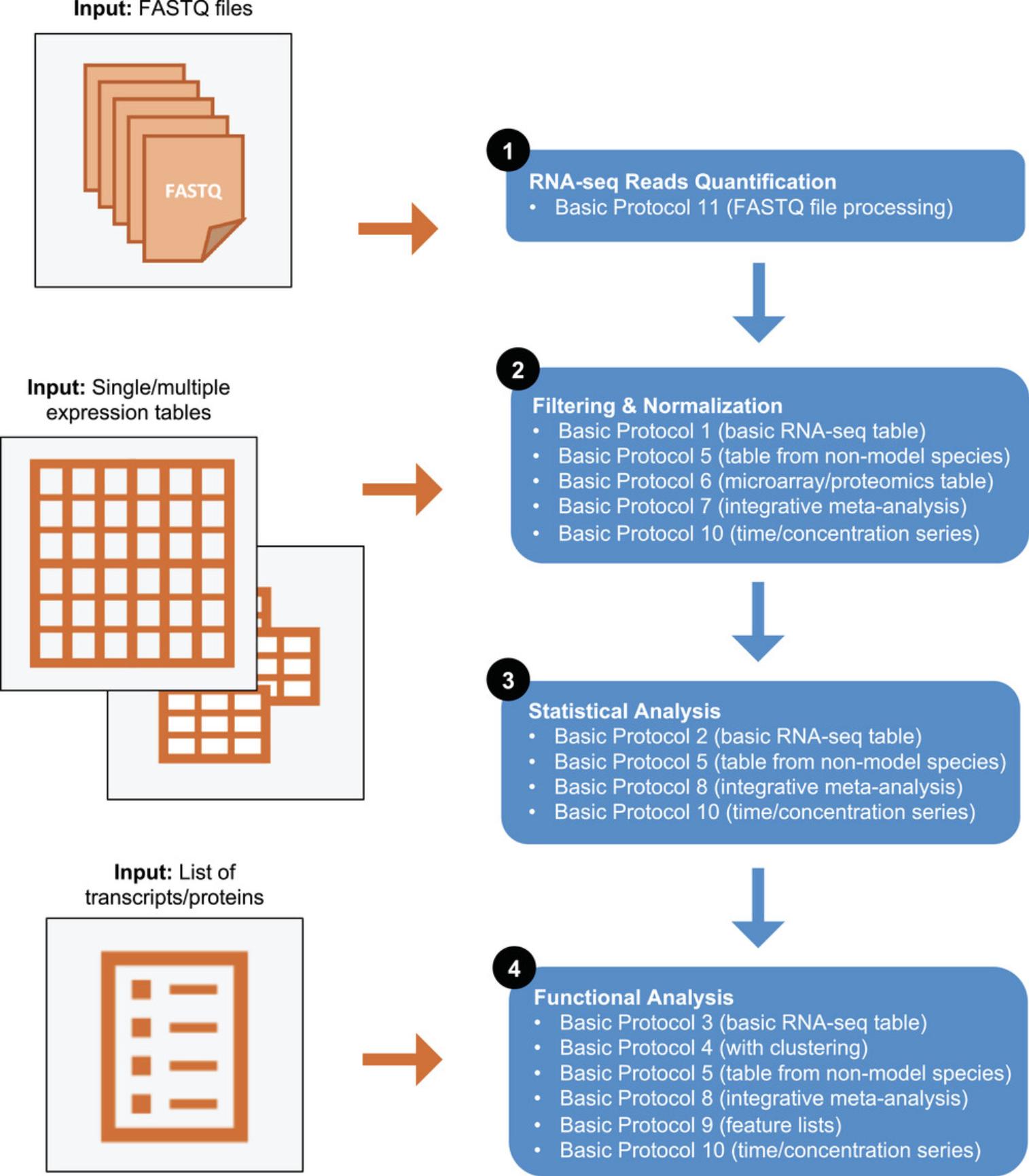
Here, we present 11 basic protocols to introduce readers to the different ExpressAnalyst modules that can be used for raw data processing, statistical analysis, and functional analysis, outlining which workflows are appropriate for model vs non-model species, transcriptomics vs proteomics datasets, and for various common data input formats. They are summarized below.
Basic Protocol 1: How to upload, process, and normalize an RNA-seq count table in preparation for statistical and functional analysis. Basic Protocol 2: How to perform differential expression analysis for simple and complex experimental designs. Basic Protocol 3: How to perform functional analysis and interpret the results with volcano plots, enrichment networks, and ridgeline charts. Basic Protocol 4: How to use hierarchical clustering and heatmaps to perform an unsupervised, exploratory analysis. Basic Protocol 5: How to perform statistical and functional analysis of a cross-species RNA-seq count table generated by ortholog mapping with Seq2Fun. Basic Protocol 6: How to filter and normalize microarray and proteomics intensity tables. Basic Protocol 7: How to upload, process, and normalize a set of gene expression tables for meta-analysis. Basic Protocol 8: How to perform statistical and functional meta-analysis of gene expression data. Basic Protocol 9: How to analyze single or multiple gene expression signatures. Basic Protocol 10: How to perform dose-response and time-series analysis. Basic Protocol 11: How to process FASTQ files to obtain a gene count table with or without using a reference transcriptome.
Basic Protocol 1: RNA-seq COUNT TABLE UPLOADING, PROCESSING, AND NORMALIZATION
The objective of this protocol is to prepare the data for downstream differential expression and functional analysis using ExpressAnalyst. This includes formatting the input files, mapping transcript identifiers to the internal annotation database, performing a basic quality check on the data, and applying filtering and normalization to remove non-informative genes and to correct for systematic technical differences. This protocol assumes that RNA-seq reads have already been aligned to a transcriptome and summarized in a count table, which is the case for most researchers. If this is not the case and you must start from FASTQ files, please see Basic Protocol 11.This protocol is also specifically written for RNA-seq count data. ExpressAnalyst also accepts abundance tables produced from microarray or proteomics experiments. Many of the overall concepts are the same; however, count data requires specific normalization techniques. For a discussion of microarray intensity and proteomics abundance data processing, please see Basic Protocol 6.
Basic Protocols 1 to 4 use the same dataset, an RNA-seq count file measured in mouse liver (Diamante et al., 2021). It has been previously shown that bisphenol-A (BPA) exposure during pregnancy leads to cardiometabolic disease in offspring. The objective of the original study was to elucidate the mode of action underlying this outcome. The authors exposed pregnant mice to BPA and collected RNA-seq data in the liver from offspring of both sexes, along with bodyweight, insulin secretion, and targeted lipids in the liver and plasma samples. Differential gene expression analysis was conducted between the exposed and control groups to understand the observed phenotypic differences and metabolic outcomes.
Necessary Resources
Hardware
- A computer with internet access
Software
- An up-to-date web browser such as Google Chrome, Mozilla Firefox, or Safari, with JavaScript enabled (see Internet Resources)
Files
- None
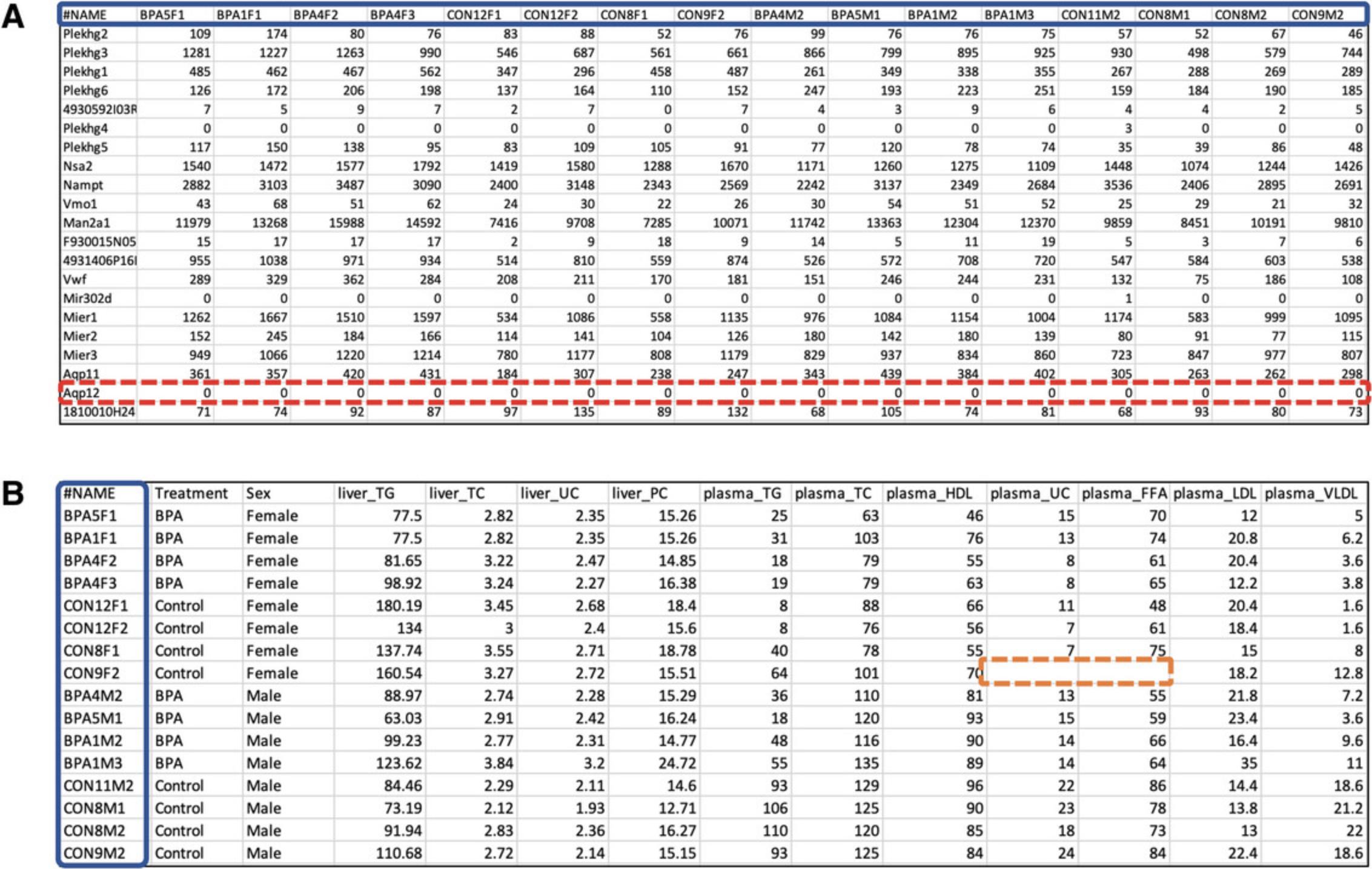
1.Go to the ExpressAnalyst home page (https://www.expressanalyst.ca) and click the “Tutorials” link at the top menu bar to visit the tutorial page. Scroll to the bottom of the page and find the “Dataset for the ExpressAnalyst Current Protocol” data section. Download the two text files labeled “mouse_counts.csv” and “mouse_metadata.csv.” Open them in a spreadsheet program or a text editor to view the data format (Fig. 2).
2.Go back to the ExpressAnalyst home page and click “Start Here” to access the Module Overview page. Locate the “Statistical & Functional Analysis” section and click the “Start Here” button underneath the single gene expression table input type. On the Data Upload page, set the organism to “ M. musculus (mouse),” leave the “Analysis Type” as “Differential Expression,” set the data type to “Counts (bulk RNA-seq),” and the ID type to “Official Gene Symbol.”
3.Choose the “mouse_counts.csv” file for the data file, and the “mouse_metadata.csv” for the metadata file. Leave the “Metadata included” box unchecked and click “Submit.” Once the upload has finished, various summary messages will be displayed in the top right corner. Click “Proceed” to view this information in more detail on the next page.
4.In the Data Quality Check page, examine the text summary of the uploaded datasets in the gray box at the top of the “Omics data overview” tab. It shows the sample size, the percentage of features that are matched to the annotation database, as well as the number and type of experimental factors.
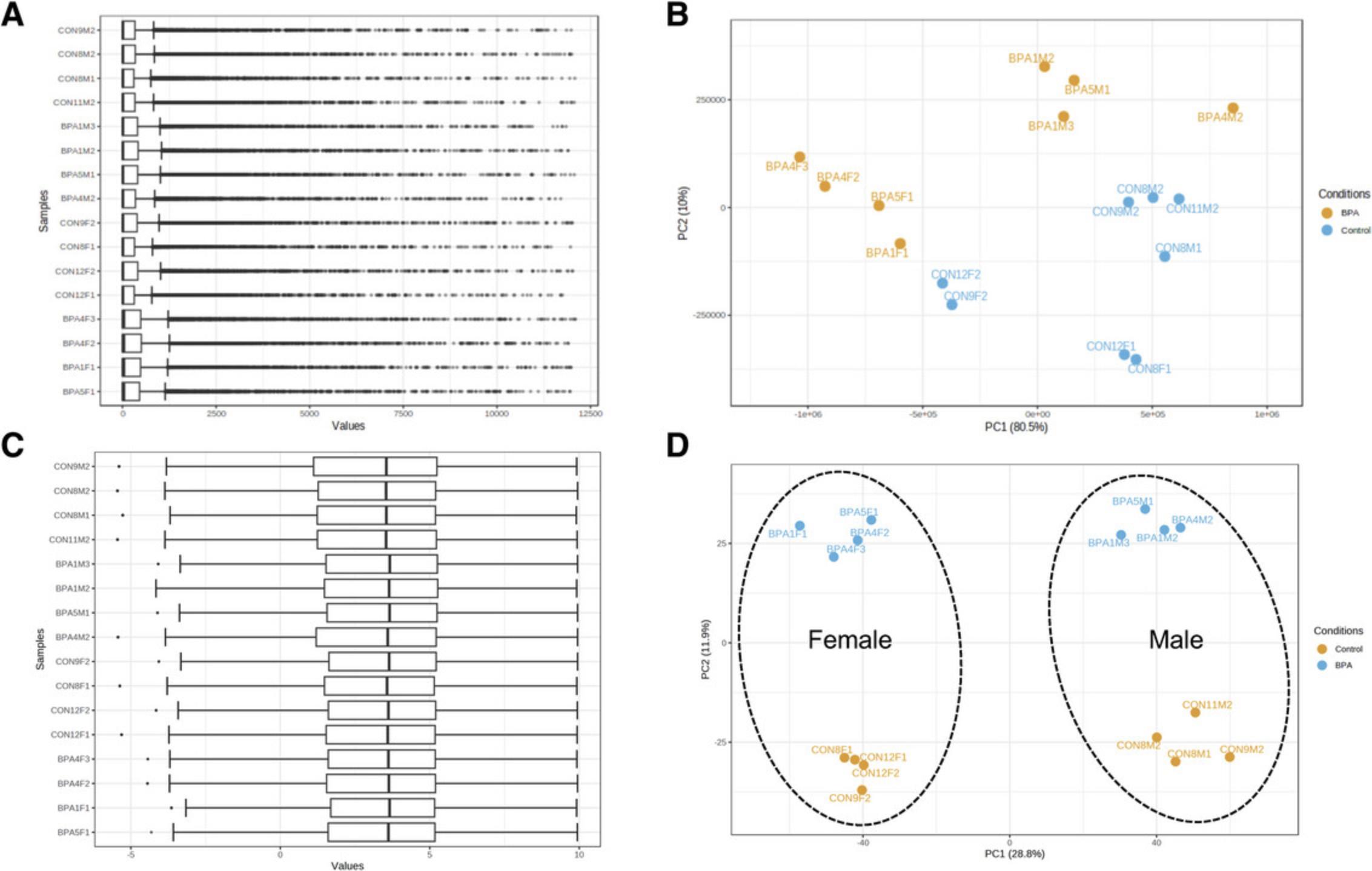
5.Scroll down to view various diagnostic graphics, the first of which is the “Box plot.” Since the expression values range from zero to >10,000, it is clear that these are unnormalized count values. Click each of the additional tabs to view the “Count sum” (displays the total counts from all genes for each sample, also called the sequencing depth), “PCA plot” (scatterplots of the top two principal components), and “Density plot” (distribution of count values for each sample) of the uploaded data. The density plot appears in the shape of an “L,” which is caused by the large range and right-skewed distribution of raw count values.
6.Go back to the top of the page and click the “Metadata overview” tab. Scroll down to the metadata table (Fig. 3) and verify that each variable has been correctly recognized as either “Discrete” (Treatment, Sex) or “Continuous” (4 liver and 7 plasma lipid variables). The classification of each metadata variable can be updated using the dropdown menus below individual variable names. Depending on your screen size, some metadata variables may not be visible. To see the additional columns, simply scroll to the right within the table area.
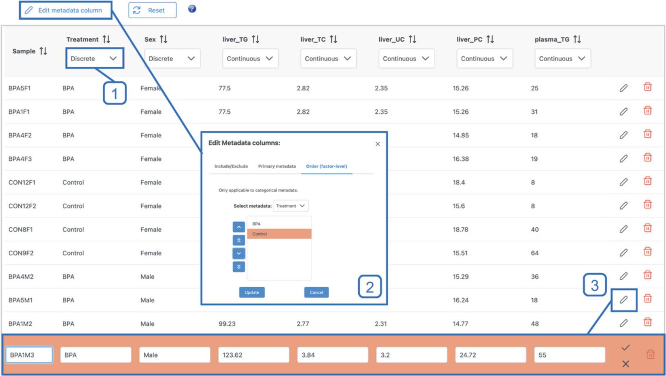
7.Click the “Edit metadata column” button above the metadata table (Fig. 3). Navigate to the “Order (factor-level)” tab and make sure the “Treatment” variable is selected in the dropdown. By default, discrete metadata classes are sorted alphabetically in all downstream plots. However, in some cases, a different order might make more sense. Here, we wish to always plot the control samples on the left and the BPA-exposed samples on the right. Click the “Control” value and use the up-arrow button on the left to move it above “BPA” and click “Update.” Click “Proceed.”
8.Click “Proceed.” A dialog will appear, warning that a few missing values were detected in the metadata and explaining how they will be handled in the downstream steps. Click “OK.”
9.Leave the default filtering settings (“Filter unannotated features” checked, “Low abundance” threshold to 4, and “Variance filter” to 15), change the normalization method to “Relative log expression normalization,” and click “Submit.”
10.Scroll down to the figures in the lower half of the page and consider the “Box plot” and “Density plot” tabs.
11.Click on the “PCA plot” tab to examine the data patterns based on principal component analysis.
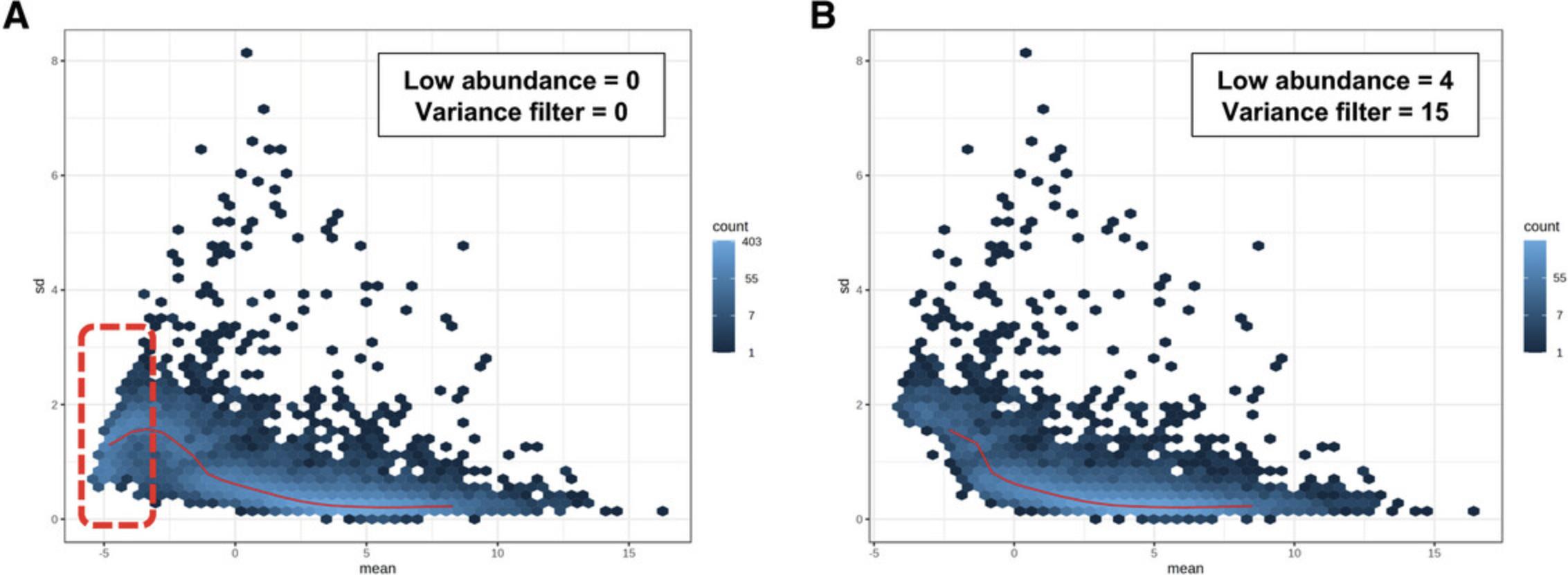
12.Click on the “Mean-variance plot” tab to explore the relationship between the mean and variance of transcript expression values.
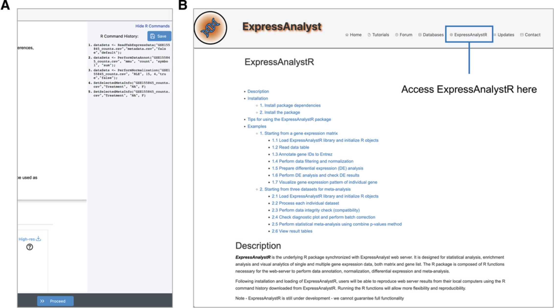
13.Click the “Show R Commands” link in the top right corner to view the R commands history.
Basic Protocol 2: DIFFERENTIAL EXPRESSION ANALYSIS WITH LINEAR MODELS
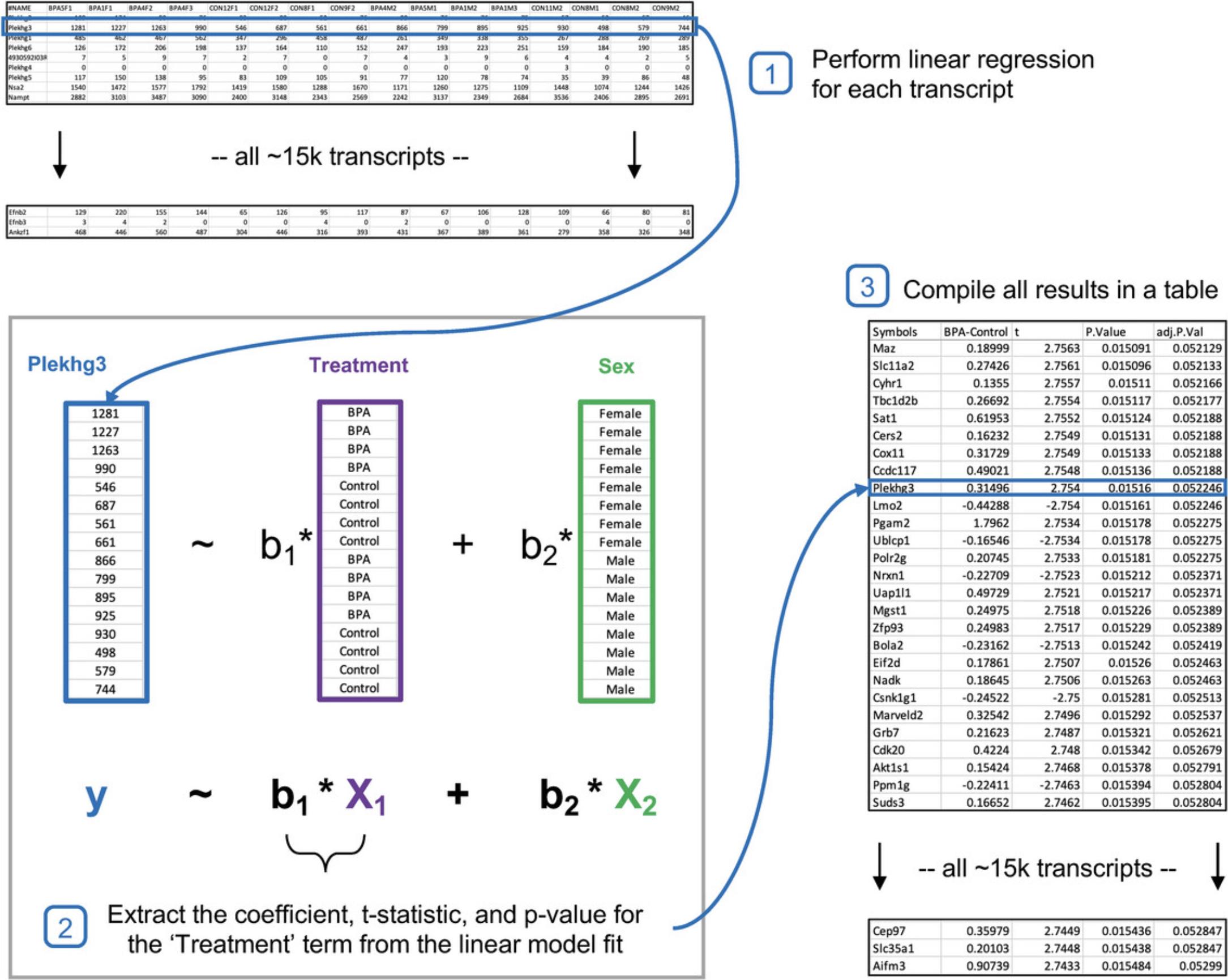
The general objective of differential expression analysis (DEA) is to identify genes or transcripts associated with specific experimental factors of interest, while accounting for other major sources of variability within the data (Law et al., 2016). The observed expression patterns can be explained by a combination of technical, biological, environmental, and experimental sources. Technical sources can include different sample preparation or sequencing depths across samples. Biological sources include factors such as sex, age, and circadian rhythm, while examples of environmental sources may encompass the geographic locations of sample collection or lifestyle parameters such as smoking or diet. Finally, experimental sources include any independent variable imposed by the researcher, such as chemical treatments or gene knockouts. In this protocol, we introduce the concepts behind using generalized linear models for performing DEA of gene expression data, explain differences between the main DEA algorithms, and describe how to configure DEA for common experimental designs.
Necessary Resources
Hardware
- A computer with internet access
Software
- An up-to-date web browser such as Google Chrome, Mozilla Firefox, or Safari, with JavaScript enabled (see Internet Resources)
Files
- None
1.This protocol carries on where Basic Protocol 1 left off. If you have not just completed Basic Protocol 1, please do so. Click “Proceed” to move from the “Data Filtering & Normalization” page to the “Differential Expression Analysis” page to begin this protocol.
2.There are two different parameter interfaces for DEA. The “Simple Metadata” tab is for datasets with only one or two discrete metadata variables, while the “Complex Metadata” tab can handle any number of metadata, including both discrete and continuous types. We will work primarily with the “Complex Metadata” interface. Click the “Complex Metadata” tab.
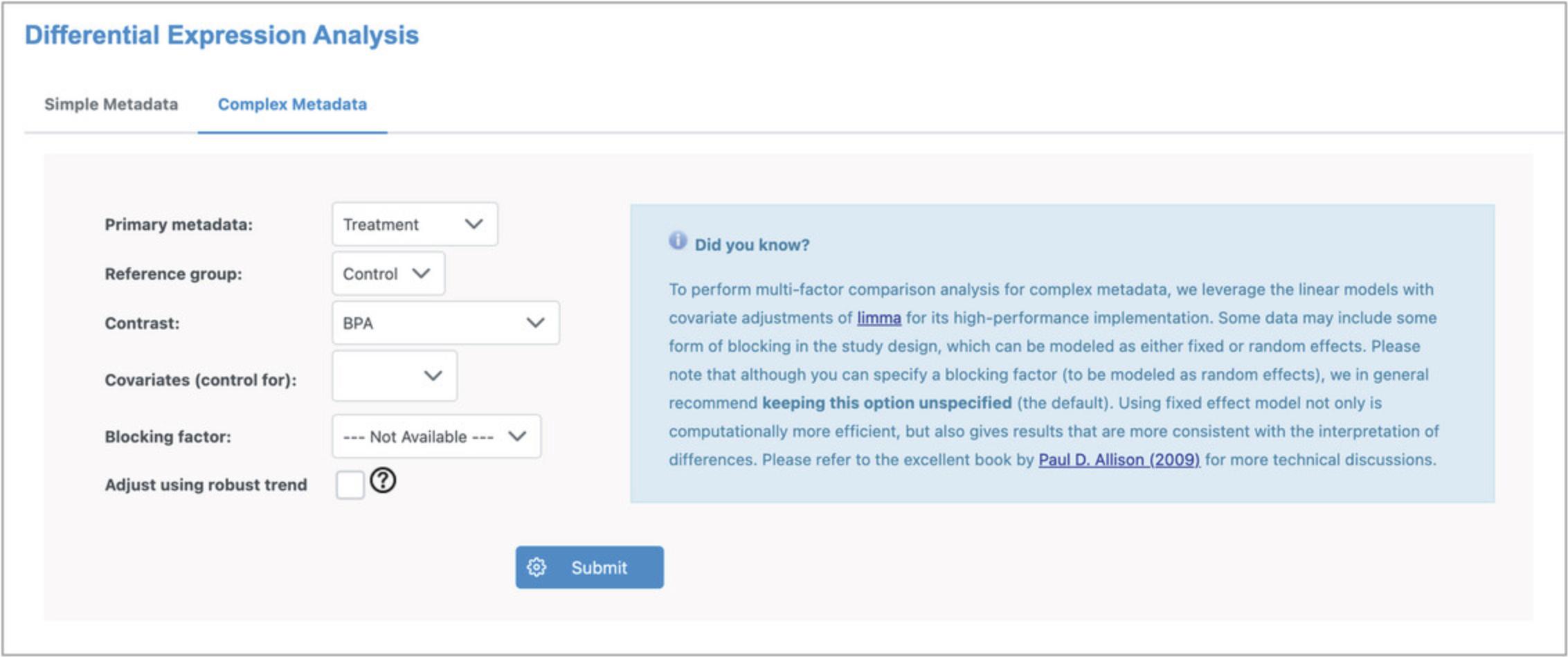
3.Change the “Reference group” to “Control” and the “Contrast” to “BPA,” leaving the remaining as the default settings. The selected parameters should be as in Figure 8.Click “Submit” and then click “Proceed.”
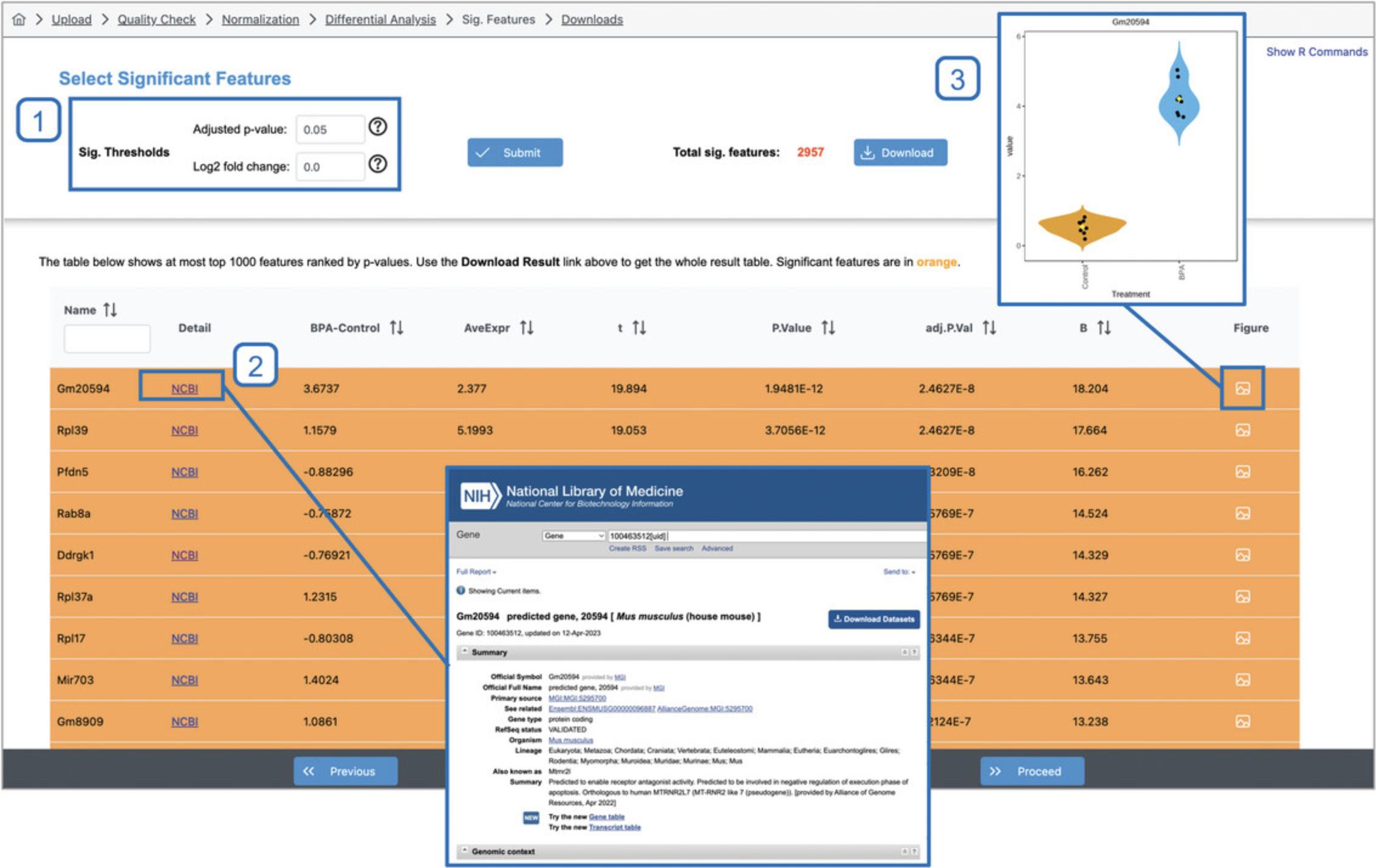
4.The simple comparison of all “BPA” samples vs all “Control” samples results in 2957 transcripts with statistically significant differences in expression values (Fig. 9). Click the image icon under the “Graphical Summary” column for the top gene (Gm20594) to view the expression values across “Treatment” groups. Click the “NCBI” link for Gm20594 to open the gene profile in the National Center for Biotechnology Information database.
5.Click “Previous” to go back to the DEA page. Instead of looking for transcripts that are differentially expressed between treatment groups, we can consider “Sex” instead. Go the “Complex metadata” tab, change the “Primary metadata” to “Sex,” change the “Contrast” to “Male,” click “Submit” and then “Proceed.”
6.Now there are 2456 significant transcripts, including those that are widely known for their sexually dimorphic expression. For example, the Xist transcript responsible for X-chromosome inactivation is the 3rd on the list. Once you are done exploring the results, click “Previous” to return to the DEA page.
7.Go to the “Complex metadata” tab. In the last few steps, we identified transcripts associated with “Treatment” and “Sex” separately. However, based on the patterns in the PCA plot that we generated in Basic Protocol 1, we expect that some transcripts are impacted by both factors, and we want to consider this in our statistical analysis. Set “Primary metadata” to “Treatment,” “Reference group” to “Control,” “Contrast” to “BPA,” and select “Sex” from the dropdown next to “Covariates (control for).” Click “Submit” and then “Proceed.” Now there are 3,801 significant features, representing a substantial increase.
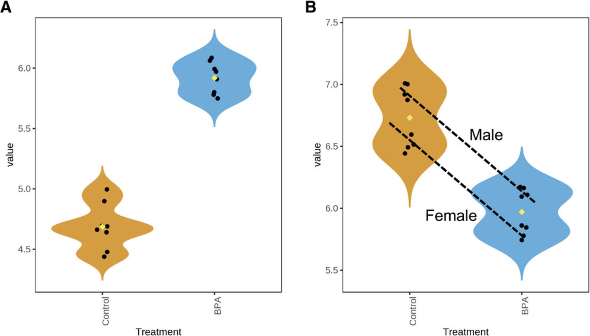
8.Click “Previous” to return to the DEA page and navigate to the “Complex Metadata” tab. Finally, we will show that continuous metadata can be analyzed as well. The metadata for this study contains measurements of four lipids in the liver and seven in the plasma, all of which are continuous (Diamante et al., 2021). While the study was designed to assess these measurements for differences between treatment groups, we can also look for transcripts associated with these values. Select ‘Liver TG’ as the primary metadata.
9.If we expect that both lipid and transcript expression levels are perturbed by BPA exposure, we may observe a significant association between some transcripts and “Liver TG.” In this case, we may naively assume that the changes in gene expression cause the changes in lipid levels, when in reality both are caused by BPA exposure, making it a confounding factor. We can avoid this by including “Treatment” as a covariate in the model. Select both “Treatment” and “Sex” as covariates, click “Submit,” and click “Proceed.”
10.There are no significant differentially expressed genes (DEGs) for this statistical comparison. This is not unexpected because this study was not designed to detect transcripts associated with the lipid concentrations. We include it to show how this type of analysis can be conducted for other datasets. Click “Previous” to return to the DEA page.
11.Click the “Simple Metadata” tab (Fig. 11). This tab allows users to choose from three different differential expression algorithms: limma , edgeR and DEseq2 (Love et al., 2014; Robinson et al., 2010; Smyth, 2005). All rely on the generalized linear model framework described above to perform DEA.
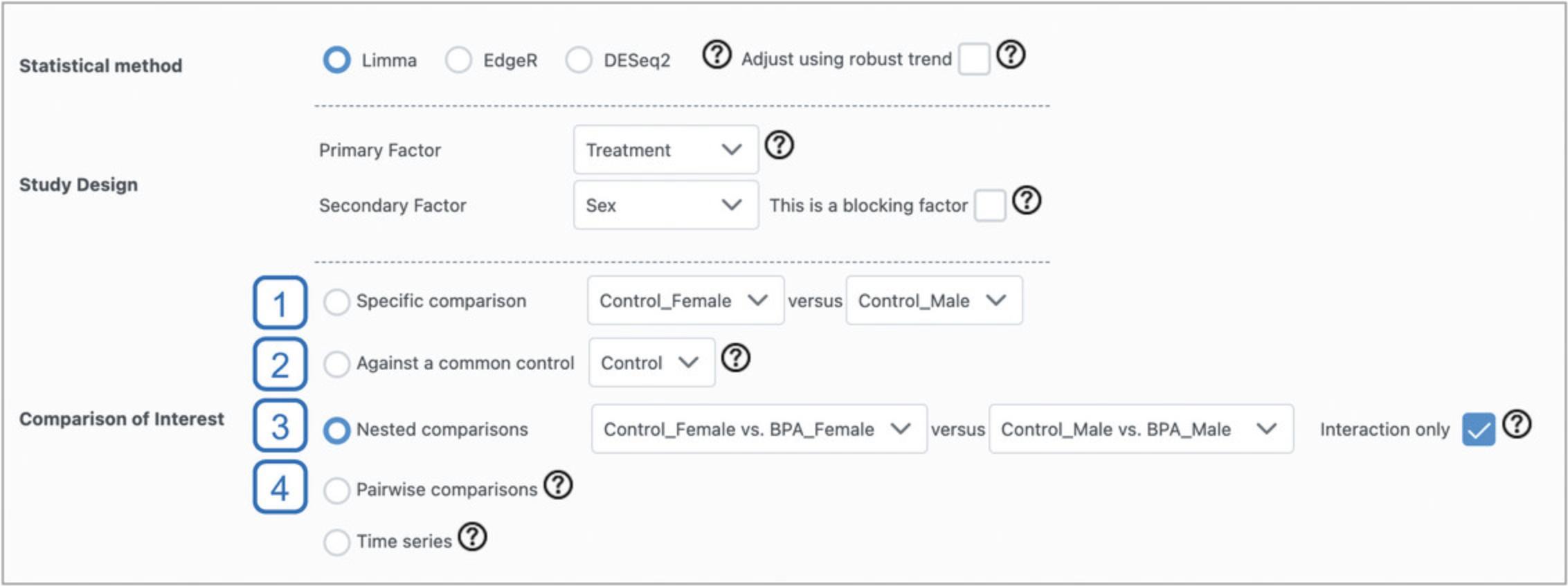
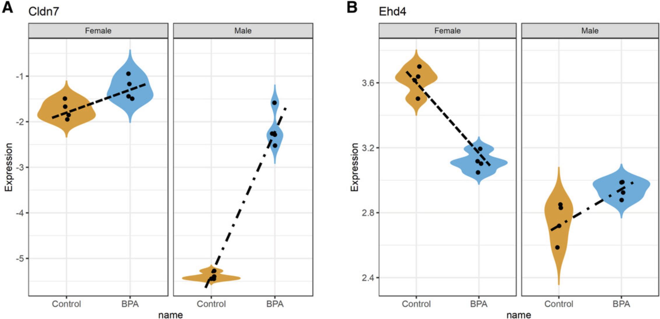
12.Leave “Limma” as the “Statistical method,” set “Primary Factor” to “Treatment” and “Secondary Factor” to “Sex.” Select the “Nested Comparisons” radio button. This allows us to specify any two comparisons between groups, and test whether the relationships defined by these comparisons are significantly different from each other. Here, we will explore whether some genes show different responses to BPA exposure between male and female mice. In the first dropdown, select “Control_Female vs. BPA_Female.” For the second dropdown, select “Control_Male vs. BPA_Male,” and check the box beside “Interaction only.” Click “Submit” and click “Proceed.”
Basic Protocol 3: FUNCTIONAL ANALYSIS WITH VOLCANO PLOT, ENRICHMENT NETWORK, AND RIDGELINE VISUALIZATION
DEA typically produces a long list (100s to 1,000s) of significant features. While specific transcripts may be meaningful to investigators, it is usually difficult to make sense of the overall biological themes within the list. Functional analysis aims to answer this question by testing whether certain functions or biological processes (encoded as different gene sets) are enriched in the gene expression data. ExpressAnalyst offers two main statistical approaches: overrepresentation analysis (ORA) (Sherman et al., 2022) and gene set enrichment analysis (GSEA) (Subramanian et al., 2005). In ORA, genes in each gene set are compared to the list of differentially expressed genes (DEGs). A gene set is considered overrepresented if the overlap is higher than we would expect from random chance. The p -value is typically computed using a hypergeometric distribution. While GSEA takes the entire list of genes (not just DEGs) ranked by some criteria (such as t-statistics or fold-changes), it then compares each gene set to the gene list and determines whether the genes in the gene set are enriched or concentrated at either the top or the bottom of the list. P -values are computed empirically using a permutation-based approach. In this protocol, we introduce three different visual analytics tools (volcano plot, enrichment network, and ridgeline chart) that can be used to perform functional analysis and visualize the results.
Necessary Resources
Hardware
- A computer with internet access
Software
- An up-to-date web browser such as Google Chrome, Mozilla Firefox, or Safari, with JavaScript enabled (see Internet Resources)
Files
- None
1.This protocol carries on where Basic Protocol 2 left off. We ended Basic Protocol 2 on a specialized statistical test that only resulted in a few DEGs. You should be on the “Significant Results” page to begin this protocol. Click “Previous” to go back to the DEA page, click the “Complex Metadata” tab, and use the same parameters as step 7 (“Treatment” - “BPA vs. Control” as primary, controlling for “Sex” as a covariate). Click “Submit” and “Proceed.” There should be 3801 significant features. Click the “Proceed” to navigate to the Visual Analytics overview page.
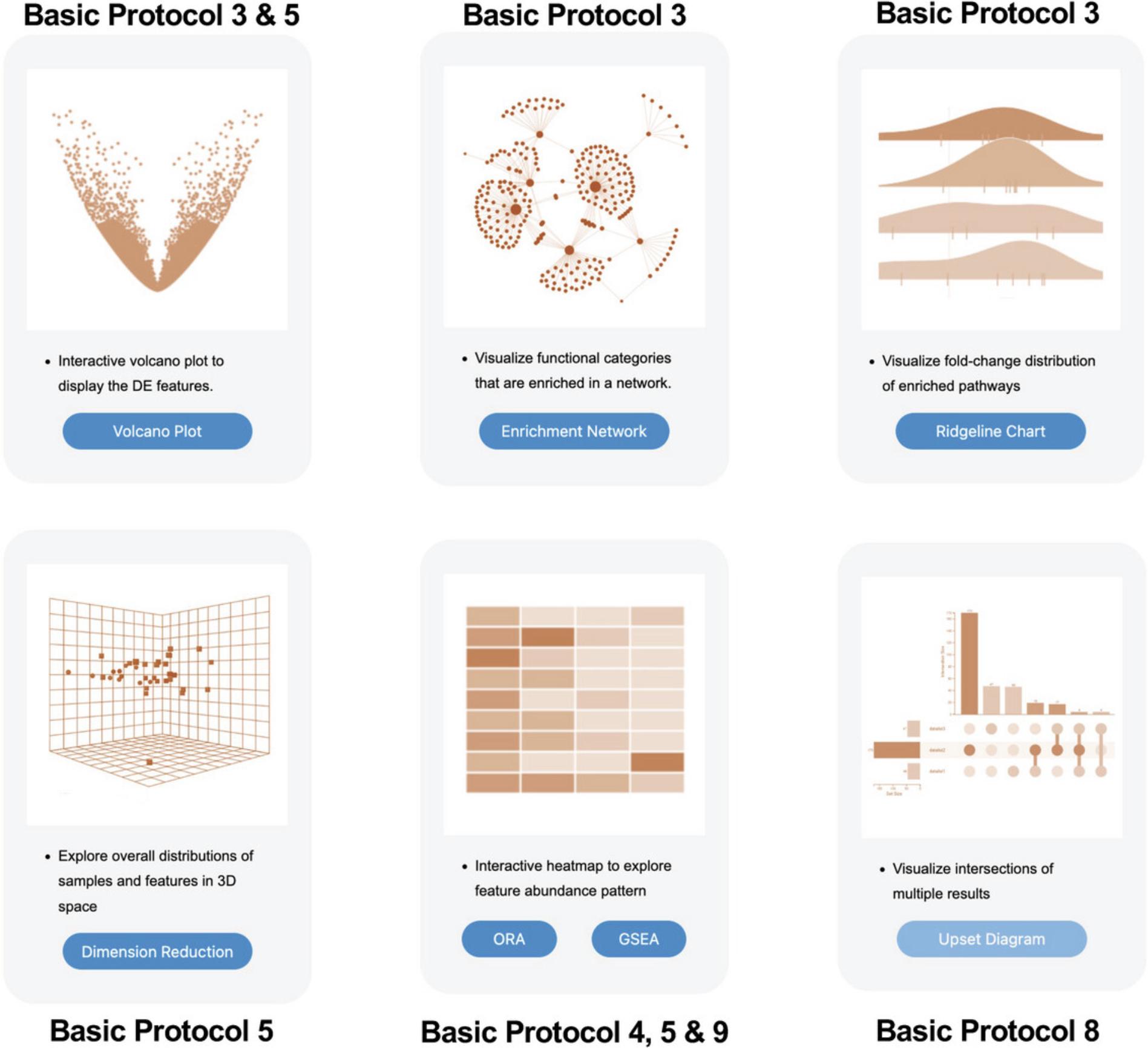
2.The “Analysis Overview” allows users to explore their data using six different interactive visual analytics tools (Fig. 13). In this protocol, we will explore the features of the three tools located in the top row. The heatmap will be covered in Basic Protocol 4 and the UpSet diagram in Basic Protocol 8.Click the “Volcano Plot” button.
3.A volcano plot that looks like Figure 14 should now appear on the screen. The log2FC values are on the x-axis, with positive values to the right and negative values to the left. The y-axis is based on -log10(p -value), so that more significant p -values will have higher y-axis values. For example, a p -value of 4.0 × 10⁻⁷ has a y-axis value of 6.4.
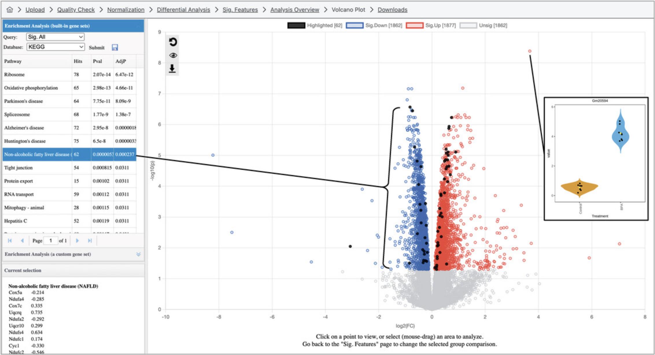
4.By default, ORA has been conducted by comparing the list of DEGs with gene sets corresponding to KEGG pathways. There are ten pathways with an adjusted p -value <0.05, although it is difficult to discern a clear overall biological theme. Both the result table and the volcano plot are interactive. As shown in Figure 14, click a row in the result table to highlight the gene members of the corresponding gene set on the volcano plot, and click a point on the volcano plot to show a box plot summary of the gene expression levels.

5.Sometimes, biological patterns are easier to interpret when we analyze the up and downregulated transcripts separately, as there are often different biological processes represented in these lists. Change the “Query” dropdown in the “Enrichment Analysis” panel on the top left to “Sig. Up” and click “Submit.” In general, we see pathways related to translation and energy generation, with pathways including “Oxidative phosphorylation,” “Ribosome,” and “Non-alcoholic fatty liver disease.” Change the “Database” dropdown to “Reactome” and click “Submit.” These significant results are more specific and follow the general pattern in the KEGG pathways with more gene sets related to the respiratory electron transport chain and translation.
6.Change the “Query” dropdown to “Sig. Down” and the “Database” dropdown to “KEGG” and click “Submit.” Here, the most significant pathways are related to transcript processing, for example “Spliceosome” and “RNA transport.” Change the “Database” to “Reactome” and click “Submit.” Just as with the upregulated transcripts, the Reactome results are related to the same themes as the KEGG pathways but are more specific and detailed.
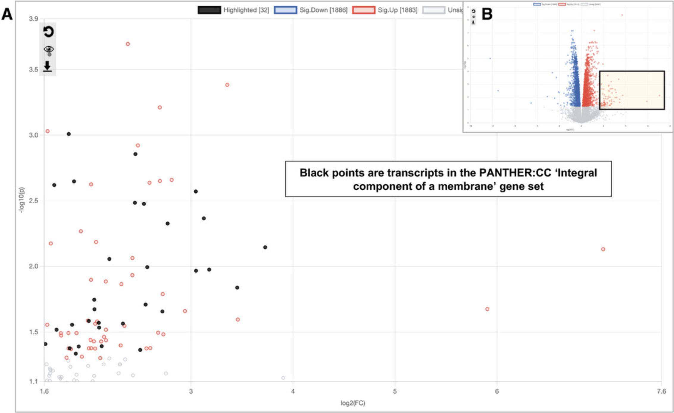
7.In the overall volcano plot, there is a group of up-regulated DEGs showing very large log2FC values (Fig. 16A). It is possible they are functionally related to each other. To investigate this hypothesis, click and drag your mouse to form a square around the transcripts highlighted in Figure 16B. This will zoom in the main plot to include only the highlighted transcripts (Fig. 16A). Next, change the “Query” to “Current View” and click “Submit” (the database should still be Reactome from the previous step). This will perform ORA with only the transcripts visible in the zoomed in volcano plot area. We see no significant results with this database. Continue exploring other gene set libraries and we notice that “PANTHER:CC” returns a significant result for “Integral component of a membrane” with ∼30 hits (the exact set of selected genes may vary depending on the precise selected area). Click the gene set row: we can now see that almost half of the visible points are highlighted (Fig. 16B).
8.Click the “Analysis Overview” link in the top navigation bar to return to the Analysis Overview page. Click “Enrichment Network.” Please be patient as this may take up to a minute to load.
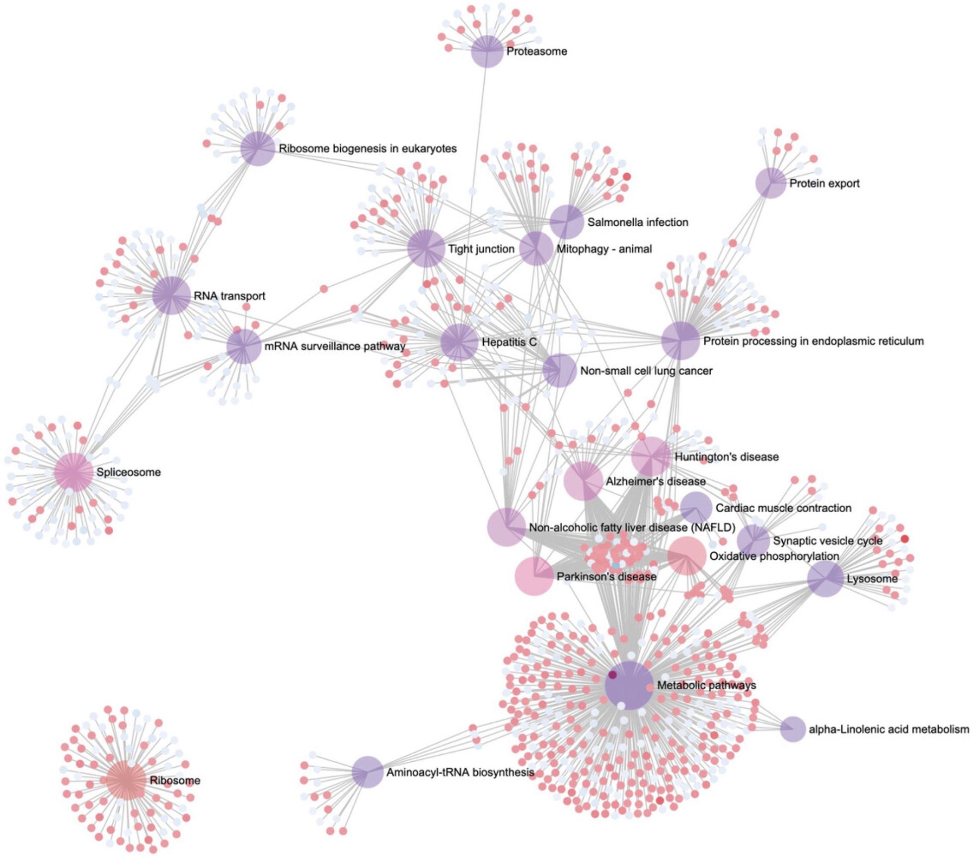
9.By default, ORA is performed with KEGG pathways, and we see that the results in the enrichment analysis panel are the same as for the volcano plot. Double-click a node in the network, such as “Synaptic vesicle cycle,” to reveal each DEG in that pathway. Double-click it again to hide the genes.
10.Go to the top toolbar and select “Bipartite Network” from the dropdown next to “View” (Fig. 17). This exposes all DEGs within each pathway. Select “Fruchterman-Reingold” from the “Layout” dropdown. Most of the network structure is visible; however, there is one section of the network where many pathway nodes are covering each other. Click and drag some of these nodes to spread them out until you can see more of the individual pathways.
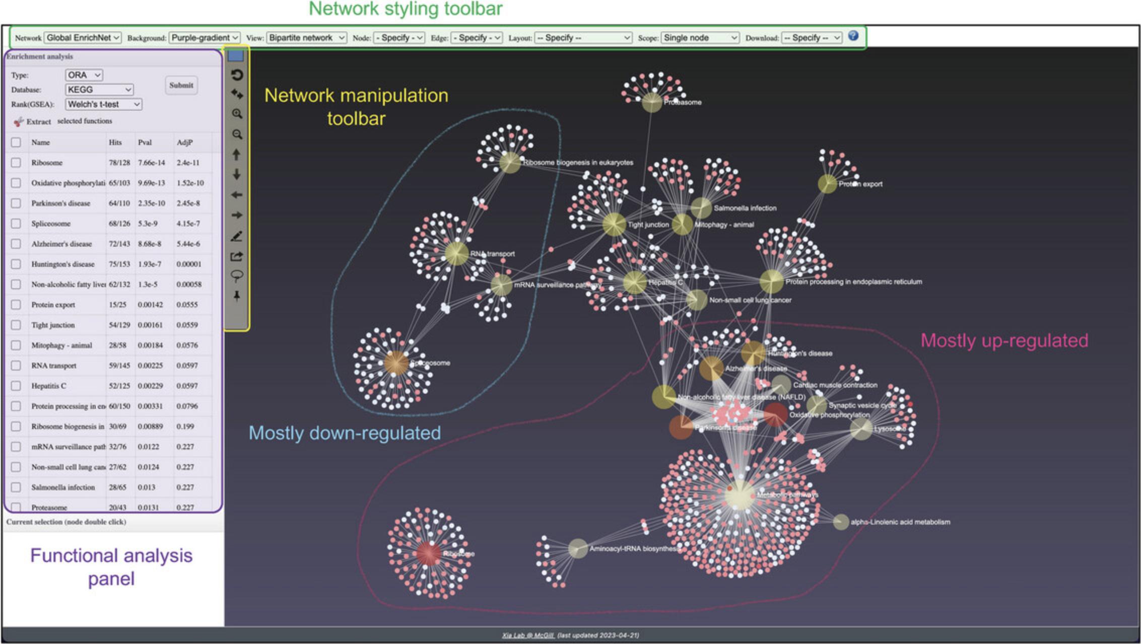
11.Images with light backgrounds are more suitable for manuscripts and publications. Select “White” from the dropdown next to “Background.” Select “PNG Image” from the dropdown next to “Download” and click “Save” in the dialog that pops up to generate and download a high-resolution version of the network suitable for publication (Fig. 18).
12.Click the “Analysis Overview” link in the top navigation bar to return to the Analysis Overview page. Click “Ridgeline Chart.” Please be patient as this may take up to a minute to load.
13.By default, ORA has been performed with KEGG pathways and the results are displayed in the “Enrichment Analysis” panel. The ridgeline diagram orders the pathways by their p -values, with the most significant at the top. The color is also related to the p -value, with darker colors corresponding to more significant p -values. The density plots show the distribution of DEGs in that pathway based on their logFC values, allowing users to see which pathways are overall up or downregulated. Each DEG is represented by a point along the baseline of each density plot. Hover your mouse over a pathway distribution to see the full pathway name, the specific p -value, and a list of all DEGs. Click a DEG point to see its expression profile.
14.In the “Enrichment Analysis” panel, change the “Type” to “GSEA,” change the “Rank” to “T-statistic” and click “Submit.” In the “Settings” panel, change “Sort by” to “Fold-change” and click “Update.”
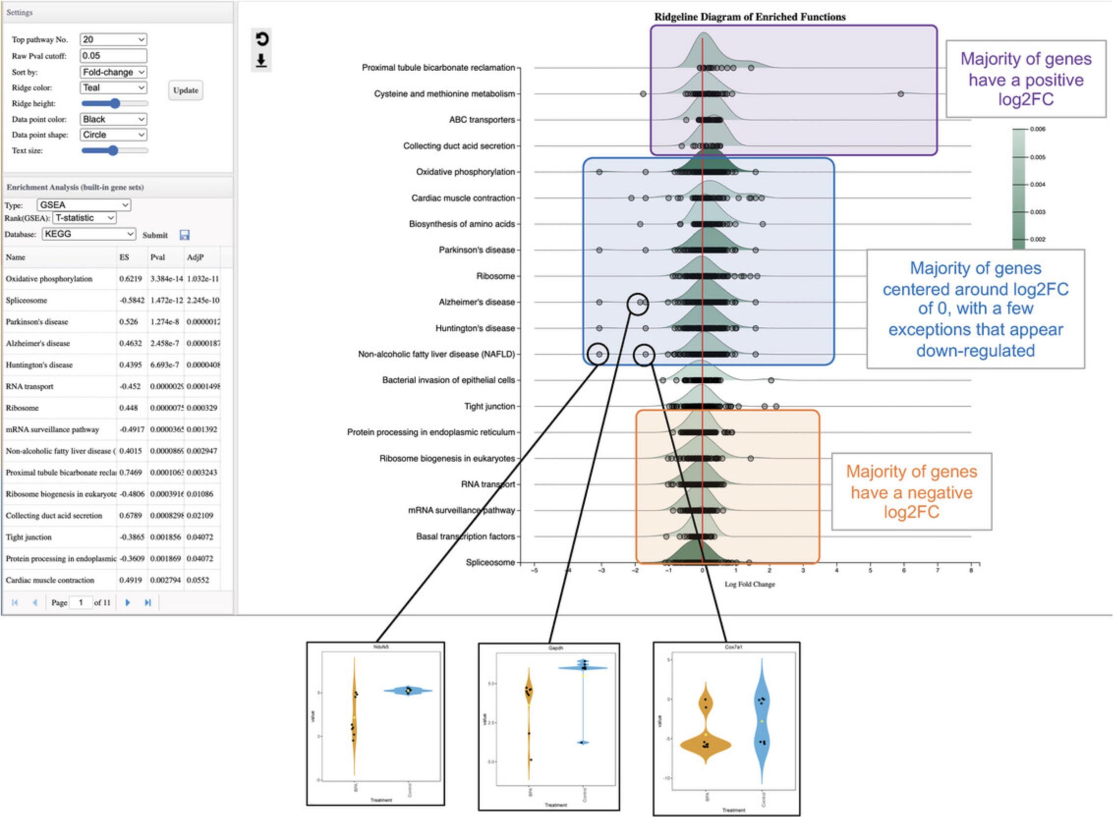
15.Click some of the gene markers in the second half of the plot that are noticeably more downregulated than the rest to investigate the expression patterns across individual samples (Fig. 19).
16.Click the “Analysis Overview” link on the top navigation bar to go back to the overview page.
Basic Protocol 4: HIERARCHICAL CLUSTERING ANALYSIS OF TRANSCRIPTOMICS DATA USING INTERACTIVE HEATMAPS
Heatmap visualization combined with unsupervised clustering is a powerful strategy for discovering and exploring gene expression patterns in transcriptomics datasets. Heatmaps display every datapoint as a colored cell, which can reveal expression patterns across different experimental factors. We can visually assess whether a DEG truly has a relatively uniform difference across all samples in each group, or if the difference was driven by a more heterogeneous response. Hierarchical clustering analysis provides an even more informative view of the data by grouping samples and genes based on their similarity to identify inherent expression patterns that are not necessarily related to their main metadata labels (D'haeseleer, 2005). The heatmap tool in ExpressAnalyst allows users to interactively select clusters of genes and perform functional analysis to help interpret any observed patterns of interest.
Necessary Resources
Hardware
- A computer with internet access
Software
- An up-to-date web browser such as Google Chrome, Mozilla Firefox, or Safari, with JavaScript enabled (see Internet Resources)
Files
- None
1.This protocol requires Basic Protocols 1 and 2 for data processing and initial statistical analysis. If you have not yet completed Basic Protocols 1 and 2, please do so first. Make sure you are on the “Analysis Overview” page to begin this protocol. Find the heatmap icon and click “ORA.” Please be patient as the heatmap may take up to a minute to load.
2.A dialogue should pop up, warning us that due to the high number of DEGs, only the top 3000 are visualized to ensure high performance of the interactive tools. Click “OK.”
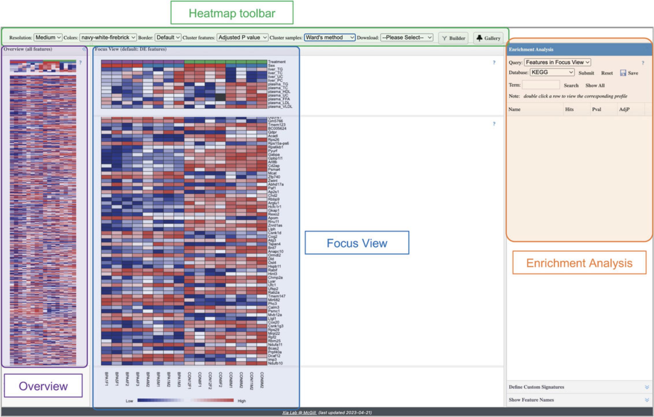
3.By default, the genes (rows) are sorted by p -value, and the samples (columns) are in the same order that they were uploaded. The top toolbar gives options for organizing the samples and genes either by metadata (samples), p -value (genes), or different hierarchical clustering methods. Locate the “Cluster Samples” option and change its value to “Treatment.” This re-arranges the samples in both the “Overview” and in the “Focus View.”
4.Change “Cluster Samples” to “plasma_TG.” Now the samples have been re-arranged again. Look at the “plasma_TG” row in the metadata section of the Focus View and notice how the “plasma_TG” cells are now arranged from dark blue to dark red (ascending order).
5.We can also use hierarchical clustering to arrange the samples. Change “Cluster samples” to “Average linkage.”
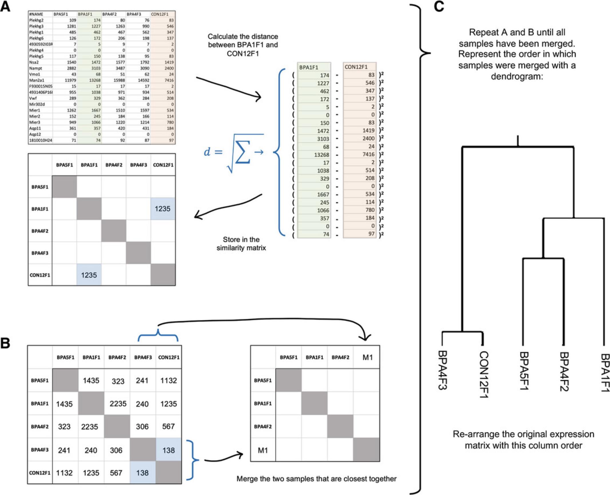
6.Now, we wil cluster genes. Change “Cluster features” to “Average Linkage.”
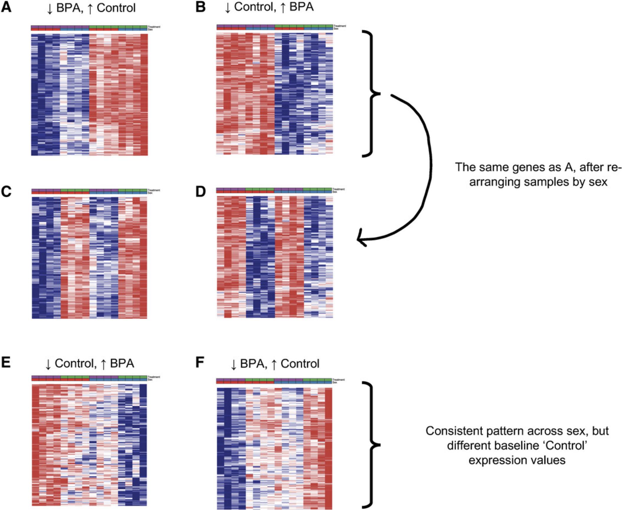
7.Scroll through the “Overview” and notice the different sections with distinct patterns (Fig. 22A and 22B). The order of the rows is no longer related to the DEA results, hence interesting clusters of genes can be present anywhere in the “Overview” heatmap.
8.Scroll to the bottom of the heatmap and find the section that matches Figure 22B (red on left; blue on right). Click and drag your mouse over the most distinct part of this section to view it in the Focus View (Fig. 23). Users can find all the gene names displayed in the current Focus View by clicking the “Show Feature Names” tab on the bottom right page.
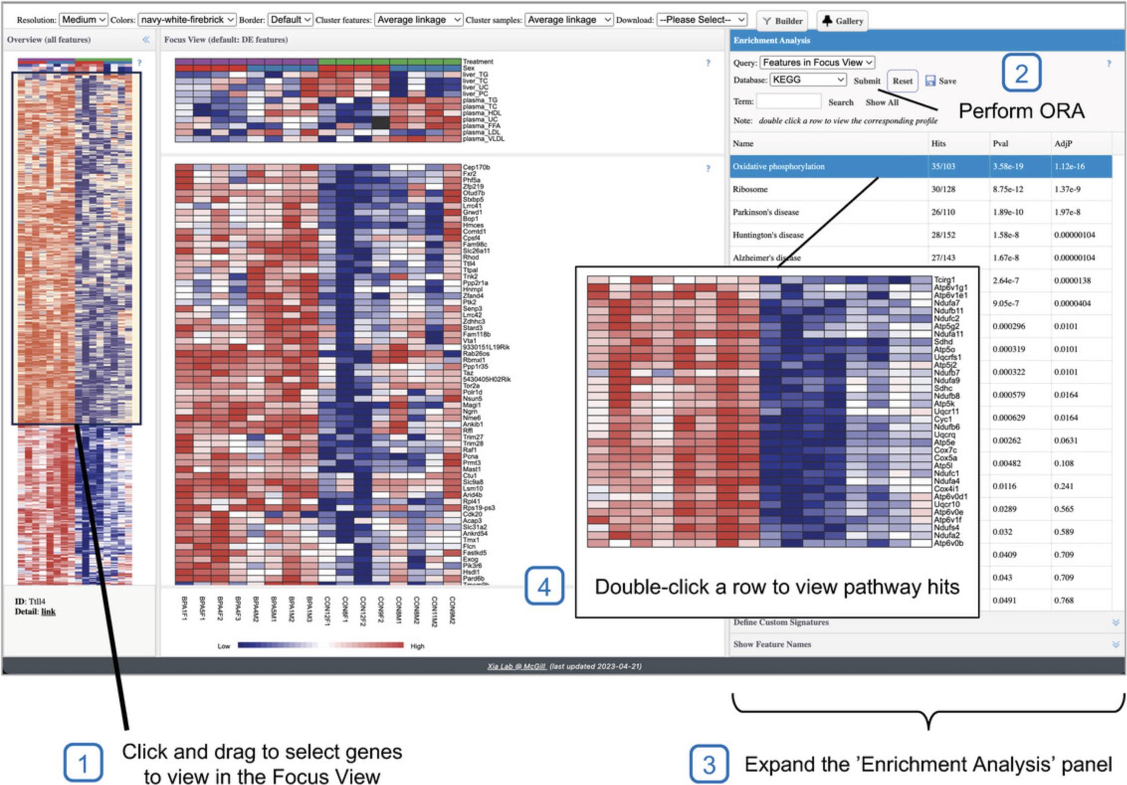
9.Go to the “Enrichment Analysis” pane, leave the defaults (Query: “Features in Focus View,” Database: “KEGG”), and click “Submit” (Fig. 23).
10.Hover your mouse over the left border of the “Enrichment Analysis” pane until it turns into an arrow pointing left. Click and drag to the left to expand the width of the “Enrichment Analysis” pane. Next, move your mouse inside of the ORA results table and find the right border of the pathway name column. Click and drag to the right until you can see the entire pathway names.
11.Double-click the top row in the results table (“Oxidative phosphorylation”) to view only those genes in the “Focus View” (Fig. 23). When you are done viewing, click the “Reset” button inside of the “Enrichment Analysis” pane to again view all the selected genes in the “Focus View.”
12.Click the “Show Feature Names” header in the right-hand panel to view the list of genes displayed in the focus view.
13.Scroll through the “Overview” to show sections with four distinct columns. It appears that these genes are related to both “Treatment” and “Sex.” Re-ordering the metadata according to “Sex” may make this easier to see. In the Focus View, double click on the heatmap row corresponding to the “Sex” to reorder. Alternatively, use the top toolbar and set “Cluster samples” to “Sex.”
14.Notice how the sections that showed uniform up or downregulation across both sexes (Fig. 22A and 22B) now look like four alternating bands (Fig. 22C and 22D). We will skip over these sections. Instead, look for the sections that look like Figure 22E and 22F. The pattern in Figure 22E shows genes that are downregulated after exposure to BPA in both female and male mice. Figure 22F shows genes that are upregulated after exposure in both sexes.
15.Select the section of genes matching the pattern in Figure 22E and perform functional analysis with several different databases.
16.Select the section of genes matching the pattern in Figure 22F and perform functional analysis with several different databases.
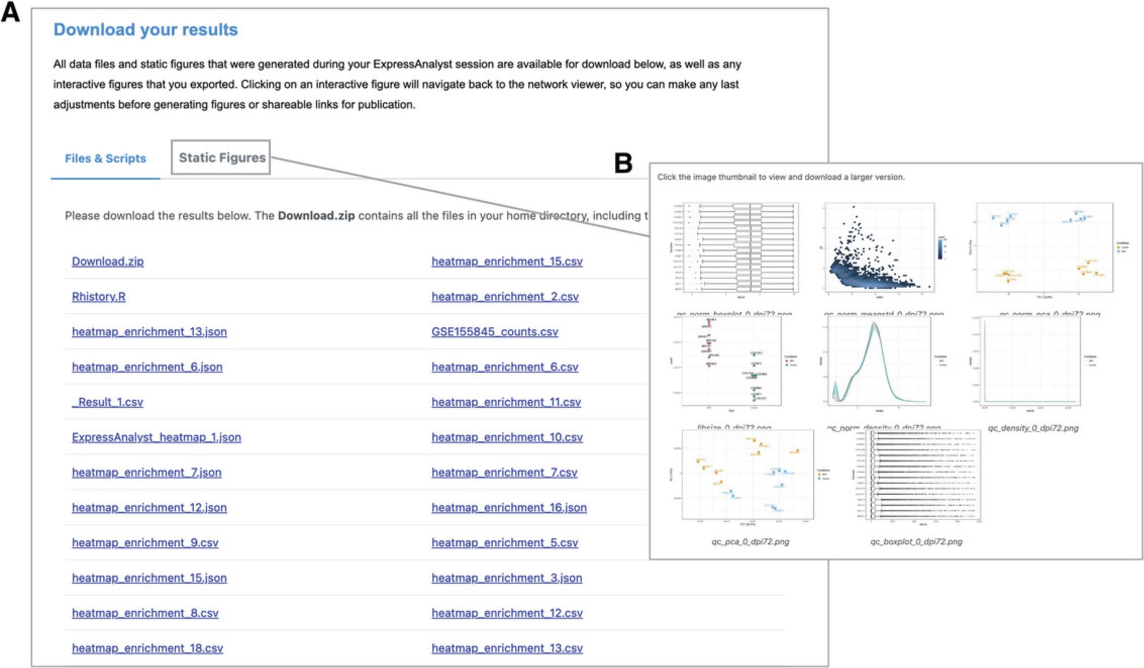
17.Go to the navigation bar at the very top of the page (above the Heatmap Toolbar) and click the “Download” link to view the results from Basic Protocols 1 to 4 (Fig. 24).
Basic Protocol 5: CROSS-SPECIES GENE EXPRESSION ANALYSIS BASED ON ORTHOLOG MAPPING RESULTS
RNA-seq analysis for non-model species can be challenging due to the lack of high-quality and well-annotated reference genomes. The Seq2Fun algorithm solves this problem by aligning short reads to a large database of protein sequences from over 600 species that have been organized into ortholog groups (EcoOmicsDB). Functional information is shared across all species to give each ortholog group a gene symbol, gene/protein description, and KEGG pathway and GO term annotations. RNA-seq reads from any species can be mapped to the same database and therefore to the same set of Seq2Fun IDs. This framework greatly simplifies comparisons of cross-species transcriptomic results compared to using reference genomes where cross-species orthologs must be first identified using BLAST. Read quantification with Seq2Fun and EcoOmicsDB is covered in Basic Protocol 11.This protocol covers statistical and functional analysis of a cross-species Seq2Fun ortholog count table. The overall workflow uses many concepts from Basic Protocols 1 to 3.Here, we focus on aspects particular to cross-species analysis with Seq2Fun results. Please refer to Basic Protocols 1 to 3 for more details on general RNA-seq data processing, statistical analysis, and functional interpretation.
The data analyzed in this protocol is from a study that aimed to identify transcriptomic signatures of tissue regeneration that is conserved across salamander species, which are able to re-grow lost limbs (Dwaraka et al., 2019). A single limb was amputated from three different species of salamanders (A. andersoni = AND, A. maculatum = MAC, A. mexicanum = MEX). A small tissue sample was collected at the time of amputation (time0) and after 24 hr (time24). There were three replicates in each species by time group, resulting in 18 total samples. One sample that appeared to be a technical outlier was removed. In this analysis, we identify genes that are consistently differentially expressed between time24 and time0 across all three species.
Necessary Resources
Hardware
- A computer with internet access
Software
- An up-to-date web browser such as Google Chrome, Mozilla Firefox, or Safari, with JavaScript enabled (see Internet Resources)
Files
- None
1.Go to the ExpressAnalyst home page and click “Start Here” to view the module overview. Find the “Statistical & Functional Analysis” section and click the “Start Here” button underneath the single gene expression table input type.
2.Click the “Try Examples” button in the bottom left of the page. Click the “Non-model organisms” link to open the data that we will analyze in a new tab.
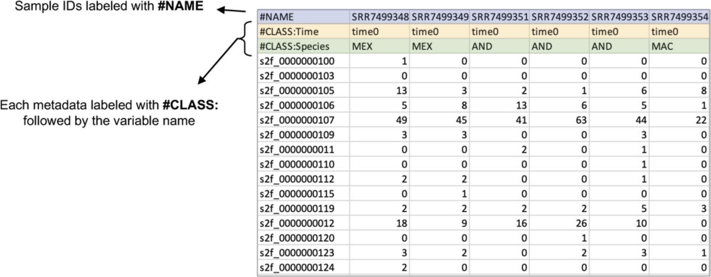
3.Select the radio button next to “Non-model organisms” and click “Submit.” When the data finishes loading, click “Proceed.”
4.As in Basic Protocol 1, we can see from the boxplot and density plot that the data are un-normalized RNA-seq counts. Click “Proceed” to go to the “Data Filtering & Normalization” page.
5.Leave the defaults (low abundance, 4; variance filter, 15; normalization, “Trimmed Mean of M-values”) and click “Submit.”
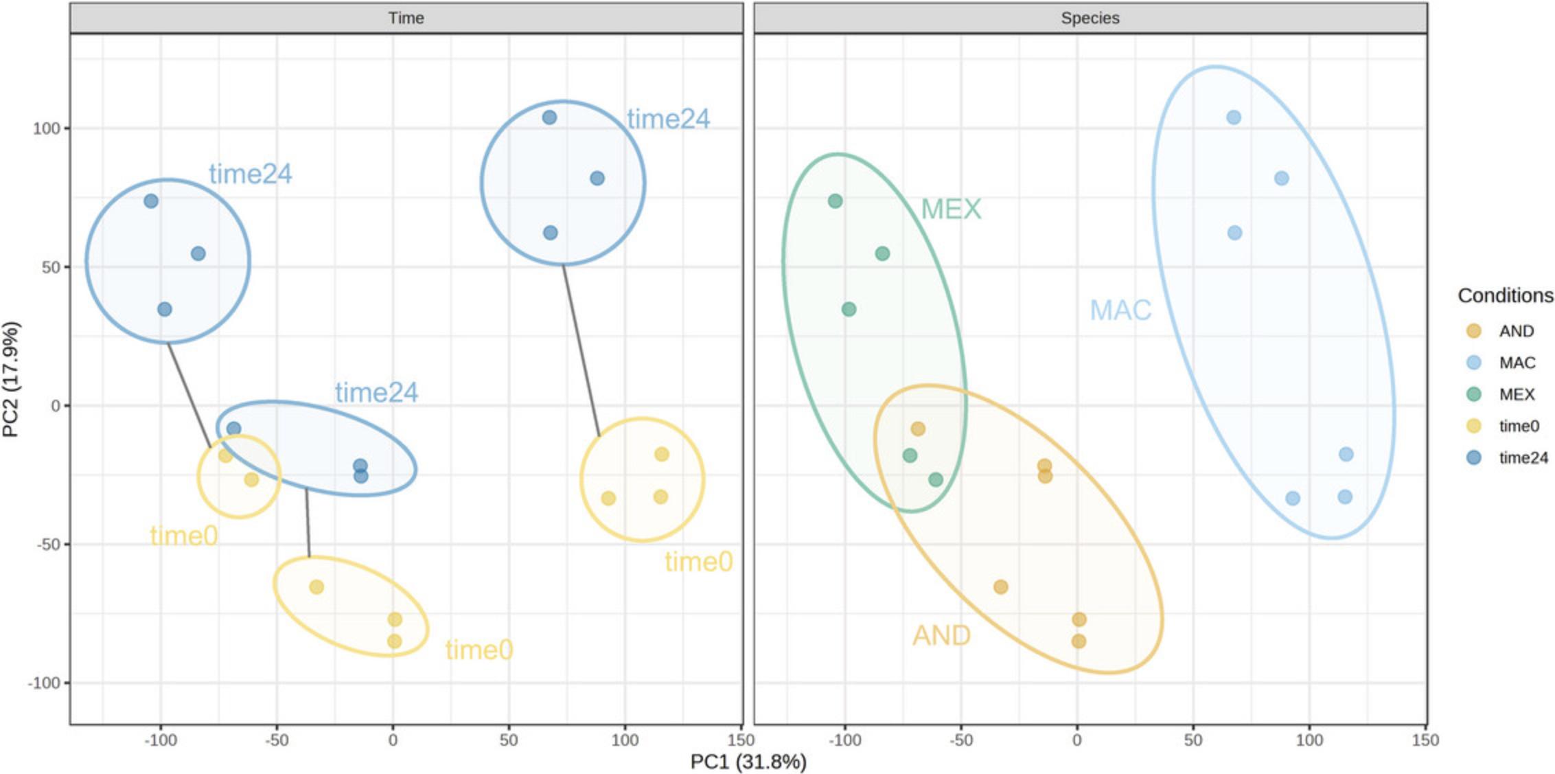
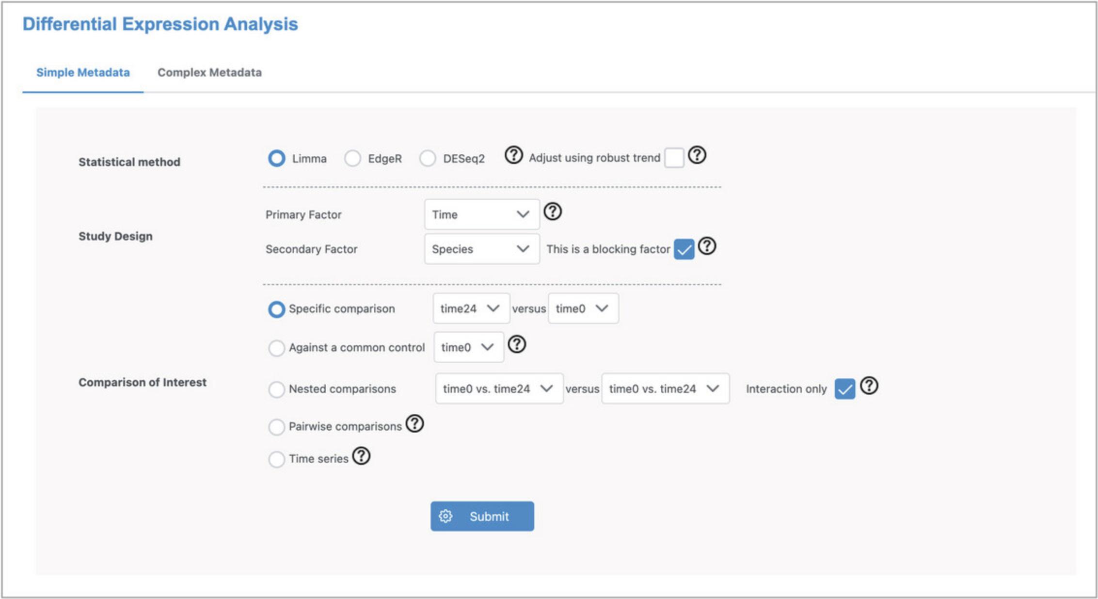
6.For DEA, we are interested in identifying a transcriptomic signature for tissue regeneration that is conserved across species. This dataset has only two categorical metadata, making it a good fit for the “Simple Metadata” tab. Stay on the “Simple Metadata” tab, leave “Limma” selected, leave “Time” as the “Primary Factor,” and select “Species” as the “Secondary Factor.” Check the box next to “This is a blocking factor.” Leave “Specific Comparison” selected but change the order in the dropdown to “time24” first and “time0” second (Fig. 27). Click “Submit” and then “Proceed.”
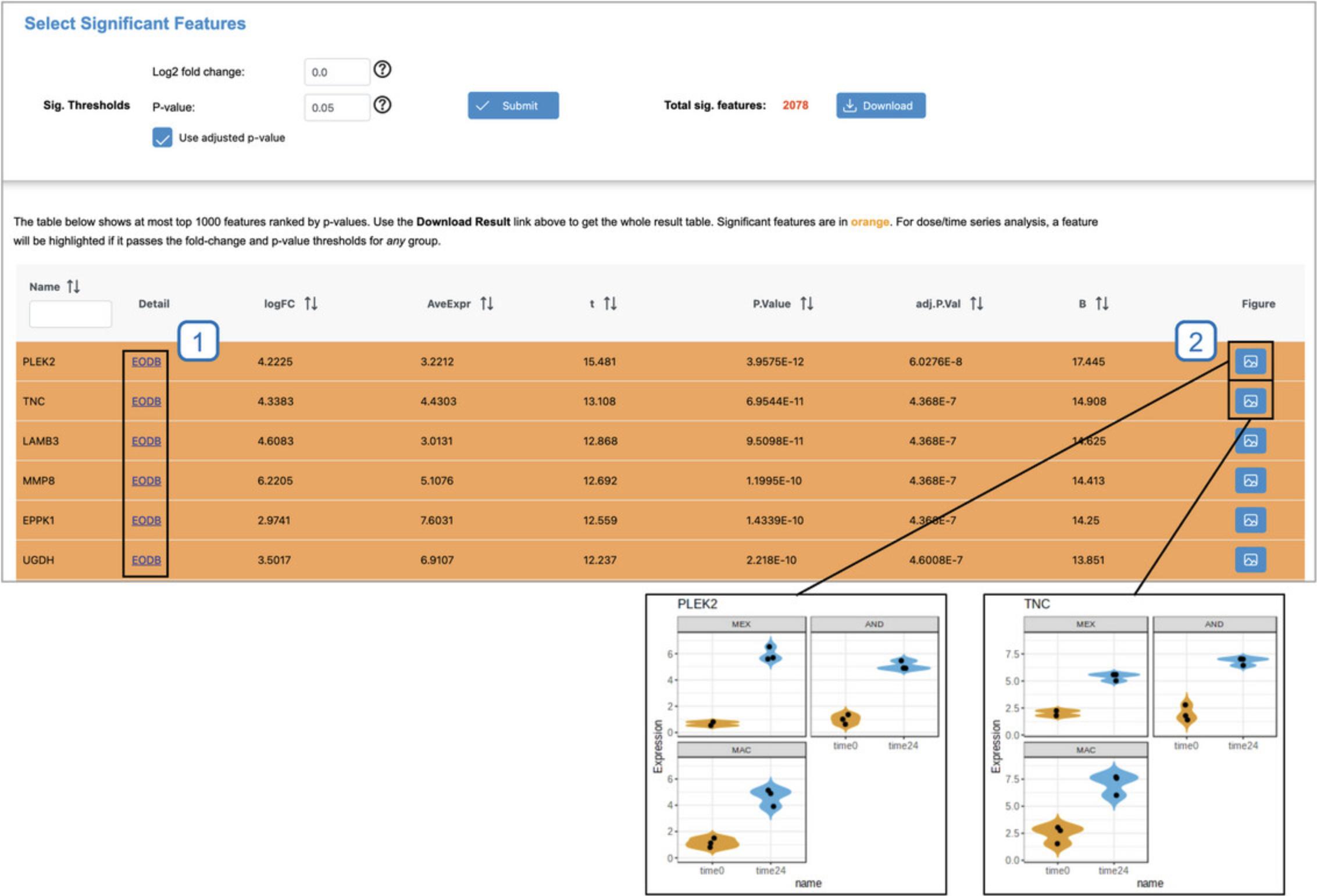
7.There are 2061 DEGs (adjusted p -value <0.05). View the expression patterns for each of the top two genes by clicking the image icon in the “Graphical Summary” column (Fig. 28). The plots clearly show that the top genes have a relationship with time that is conserved across species.
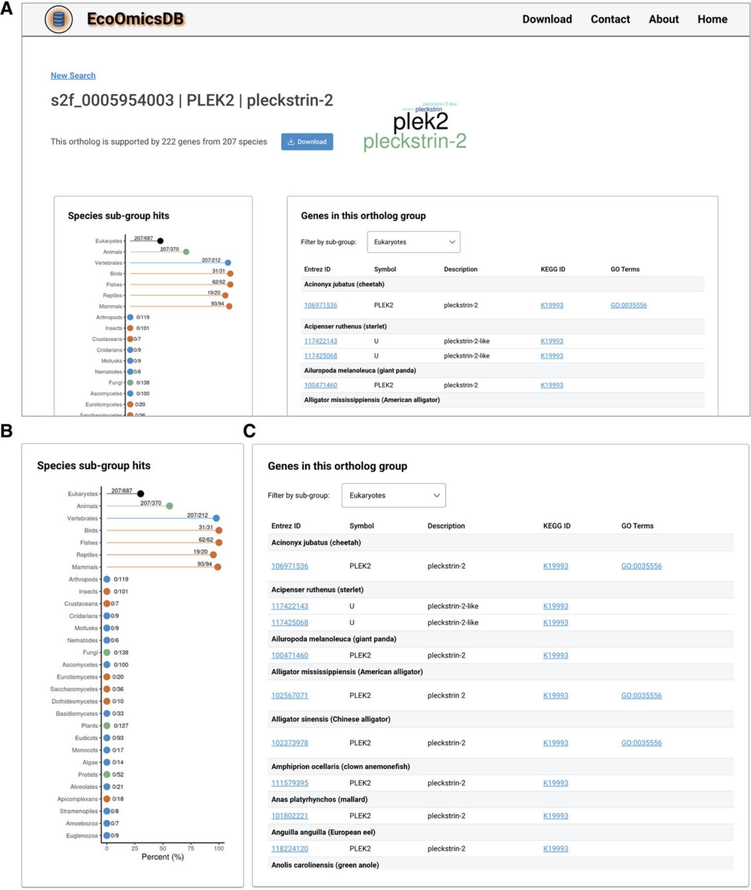
8.Click the “EODB” link for the most significant gene (PLEK2) to open the Seq2Fun ortholog profile in EcoOmicsDB.
9.Ensure that you are on the “Select Significant Features” page in ExpressAnalyst. Click “Proceed” to go to the “Analysis Overview” and then click “Volcano Plot” to perform functional analysis.
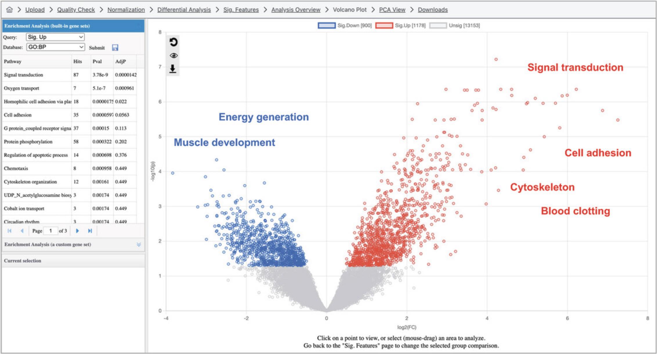
10.Go to the “Enrichment Analysis” panel and change the query to “Sig. Up,” the database to “GO:BP” and click “Submit.” This will perform ORA on the list of DEGs with positive log2FCs. After examining the results, change the query to “Sig. Down” and click “Submit” again to perform ORA on the list of DEGs with negative log2FCs (Fig. 30).
11.Click the “Analysis Overview” at the top navigation bar, and then click “Dimension Reduction.” Please be patient as it may take up to a minute to load.
12.The “Settings” panel in the top left of the screen allows users to adjust the appearance of the 3D scatterplot. Change the background to white by clicking the box next to “Background” (#1 in Fig. 31A). Click the box next to “Floor” and change it to a lighter gray. Select the checkbox next to the box (#2 in Fig. 31A). Select the checkbox next to “Shadow” (#3 in Fig. 31A).
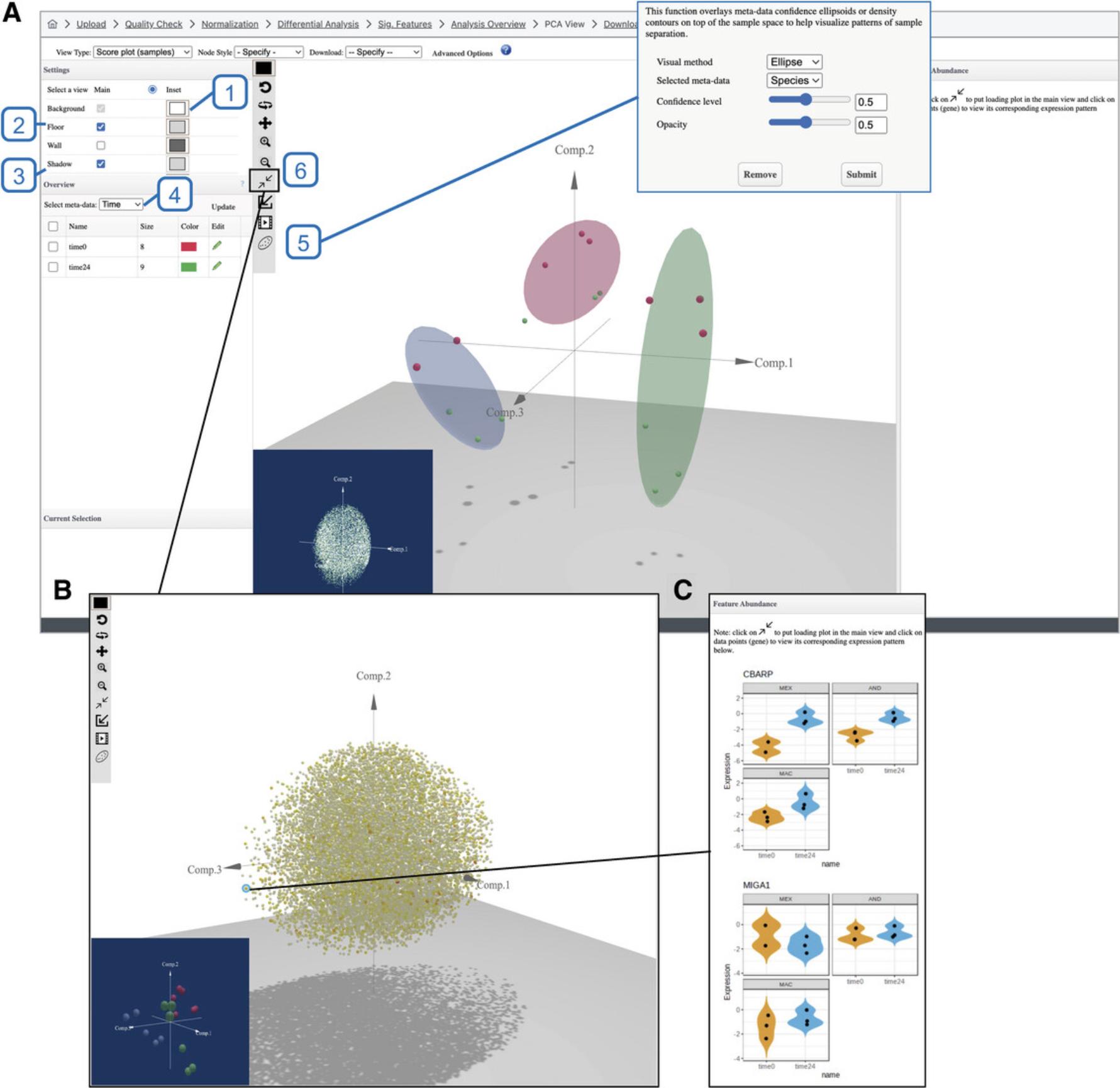
13.By default, the points are colored according to their “Time” annotation. We want to distinguish points based on “Species” annotation. First, go to the “Overview” panel and change the “Select meta-data” dropdown from “Time” to “Species” (#4 in Fig. 31A) and click “Update.” Go to the vertical toolbar inside of the plot view and click the icon that looks like an oval around some points (#5 in Fig. 31A). In the dialog, make sure that the “Selected meta-data” is “Species” and click “Submit.” Go back to the “Selected meta-data” dropdown in the “Overview” panel and change it back to “Time” and click “Update.”
14.Go to the vertical toolbar and click the icon that looks like two arrows pointing to each other (#6 in Fig. 31A) to change the view from the scores plot to the loading plot (Fig. 31B). If the ellipsoids are still present in the loading plot, click the icon that looks like an oval around some points and click “Remove” in the pop-up dialog to remove them. Click one of the points on the extreme range of the sphere to display the feature plot (Fig. 31C).
15.Navigate back in your browser to return to the “Analysis Overview,” find the heatmap and click “GSEA.” Leave “Fold-change” and “Multi-level (recommended)” selected in the GSEA Parameter Setting dialog and click “Proceed.” Please be patient as it may take up to a minute to load.
16.By default, GSEA has been conducted with KEGG pathways (Fig. 32). The most significant pathway is selected. Go to the top Heatmap Toolbar and set “Cluster features” to “Ward's method” to cluster genes based on the similarity of their expression profiles. Select different pathways to see their expression profiles.
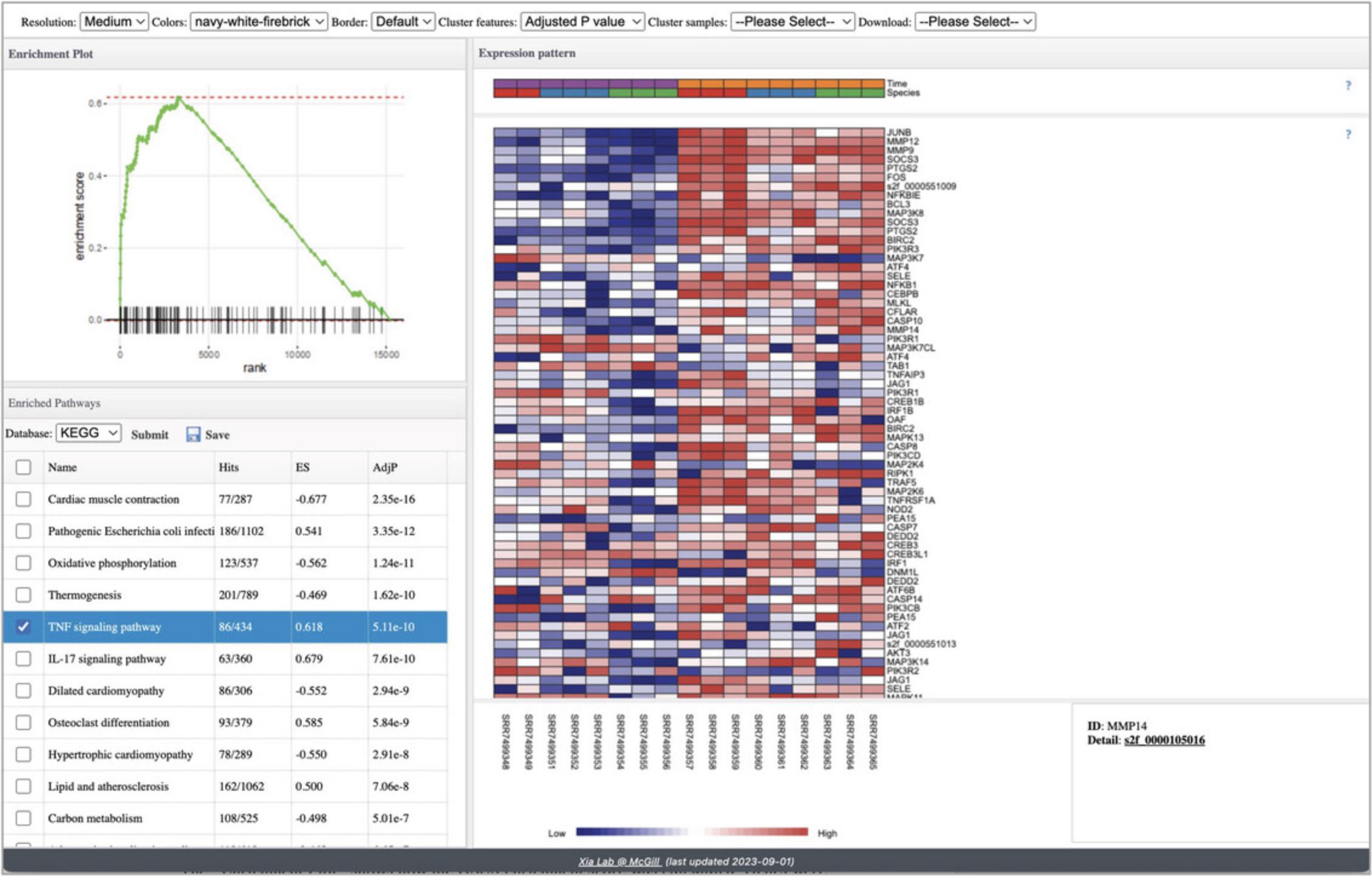
17.Click the checkbox next to “TNF signaling pathway” to view this pathway.
18.Go to the navigation bar at the very top of the page and click the “Downloads” link to view and download the results.
Basic Protocol 6: PROTEOMICS AND MICROARRAY DATA PROCESSING AND NORMALIZATION
Basic Protocols 1 to 4 covered the steps for a standard RNA-seq data analysis workflow. Proteomics and microarray data are both intensities rather than counts and should be processed differently. However, once the intensity data are properly normalized, the statistical and functional analysis pipelines introduced for RNA-seq data can be used to analyze the proteomics and microarray data.
Even though proteomics and microarray data are both intensity values, they differ in some key respects. Proteomics data generated using liquid chromatography mass spectrometry (LC-MS) tend to have more missing values than microarray data, and the workflows usually have an imputation step to avoid filtering out a high number of features (Lazar et al., 2016). The dynamic range of LC-MS is greater than that of microarray data. For these reasons, specialized normalization methods have been developed for each data type. In this protocol, we will briefly go through data upload, annotation, filtering, and normalization for a proteomics and microarray dataset. After these steps, the methods in Basic Protocols 2 to 4 can be used to perform statistical and functional analysis.
Necessary Resources
Hardware
- A computer with internet access
Software
- An up-to-date web browser such as Google Chrome, Mozilla Firefox, or Safari, with JavaScript enabled (see Internet Resources)
Files
- None
1.Go to the ExpressAnalyst home page (https://www.expressanalyst.ca) and click the “Tutorials” link at the top menu bar to visit the tutorial page. Scroll to the bottom of the page and find the “Dataset for the ExpressAnalyst Current Protocol” data section. Download the two text files “microarray_example.csv” and “proteomics_example.csv” from the download link under “Basic Protocol 6 (microarray and proteomics).” These data were previously published in two different studies (Su et al., 2002; Wigger et al., 2021).
2.Go to the ExpressAnalyst home page and click “Start Here” to view the module overview. Find the “Statistical & Functional Analysis” section and click the “Start Here” button underneath the single table input type.
3.Start with the microarray example data and select “human” for organism, keep the analysis type as “Differential Expression,” select “Intensities (microarray)” for the data type, and select “Affymetrix Human Genome U95 (chip hgu95a)” for the ID type. Select the “microarray_example.csv” file, check the “Metadata included” box, click “Submit” and then “Proceed.”
4.Examine the “Omics data overview” and the diagnostic plots at the bottom of the page. When you are done, click “Proceed.”
5.Leave the filtering settings as the defaults. Please refer to Basic Protocol 1 step 9 for an explanation of the filtering step; the principles are the same for microarray and RNA-seq data. There are five different normalization options. Select “None” and click “Submit,” to see what the data looks like without any normalization.
6.Select “Quantile Normalization” and click “Submit.”
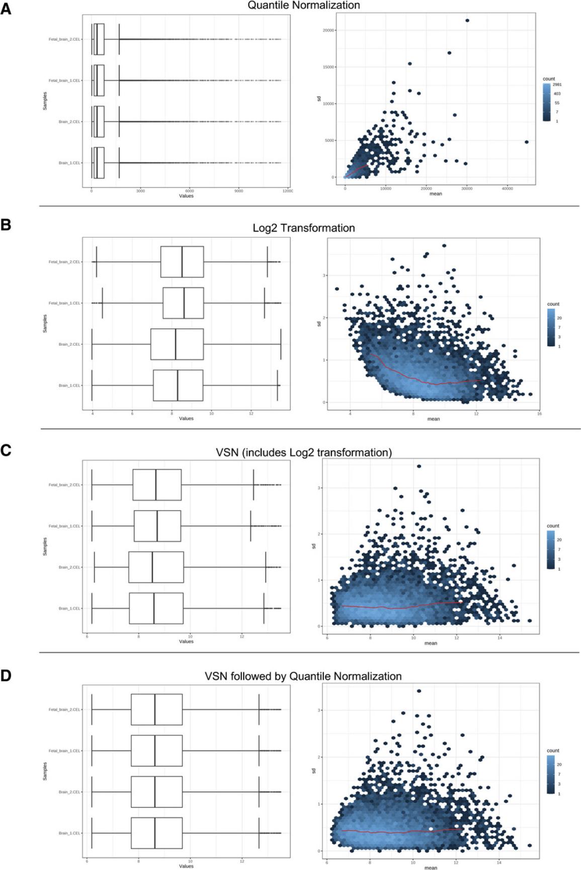
7.Select “Log2 Transformation” and click “Submit.”
8.Select “Variance Stabilizing Transformation (VSN)” and click “Submit.”
9.Select “VSN followed by Quantile Normalization.”
10.Go back to the ExpressAnalyst home page and click “Start Here” to view the module overview. Find the “Statistical & Functional Analysis” section and click the “Start Here” button that is underneath the single table input type.
11.Select “Human” for the organism, “Intensities (proteomics)” for the data type, leave the analysis type as “Differential Expression,” and set “Official Gene Symbol” for the ID type. Select “proteomics_example.csv” for the omics data file and check “Metadata included.” Click “Submit” and “Proceed.”
12.View the “Omics data overview.”
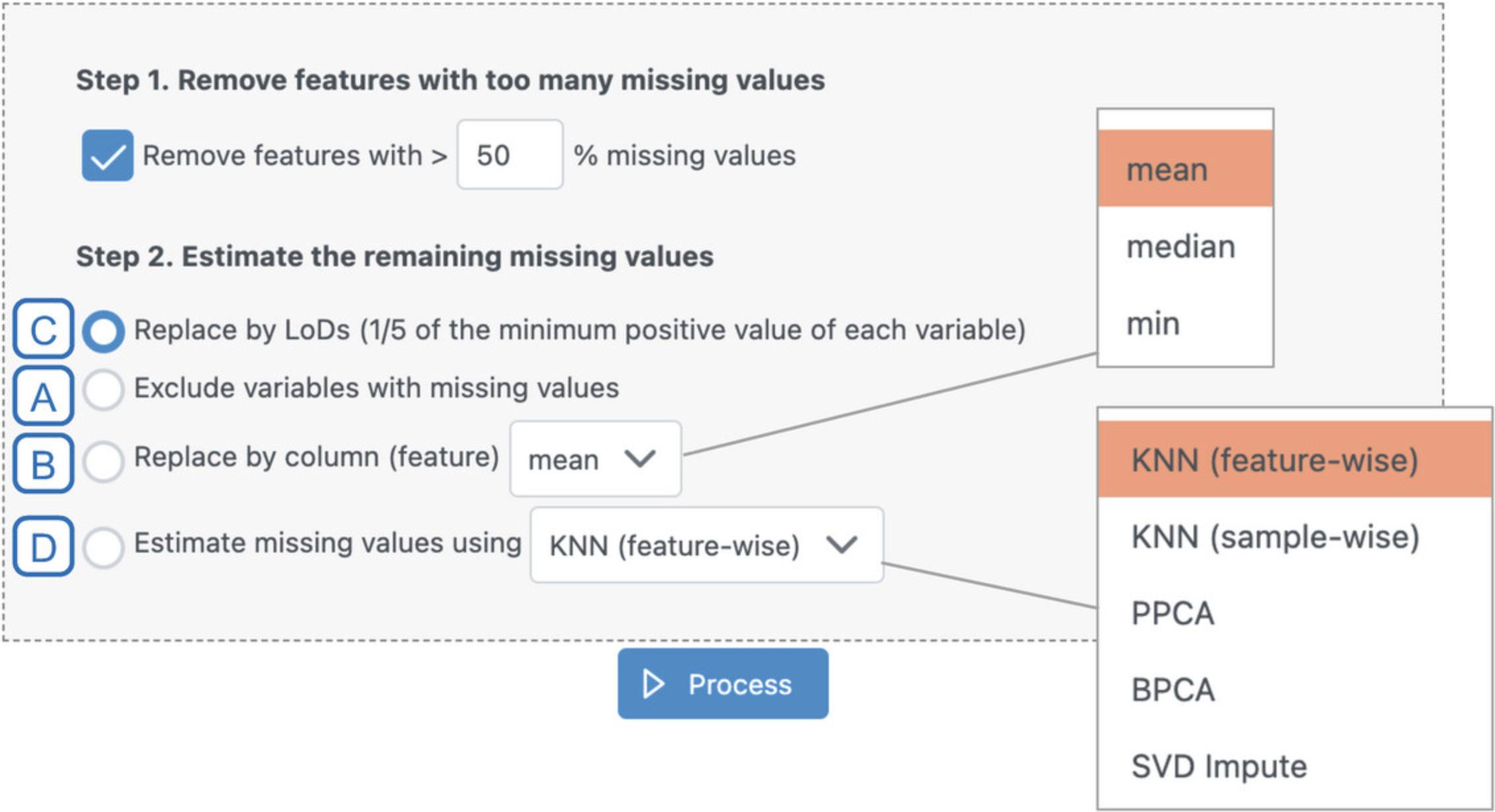
13.Navigate to the “Missing value estimation” tab. Leave “Remove all features with >50% missing values” checked. Select the last radio button “Estimate missing values using KNN (feature-wise).” Click “Process” and then “Proceed.”
14.Since we already have relatively few features (<3000), set both the abundance and variability filters to 0. Select “None” for the normalization method and click “Submit,” to see what our unnormalized data look like.
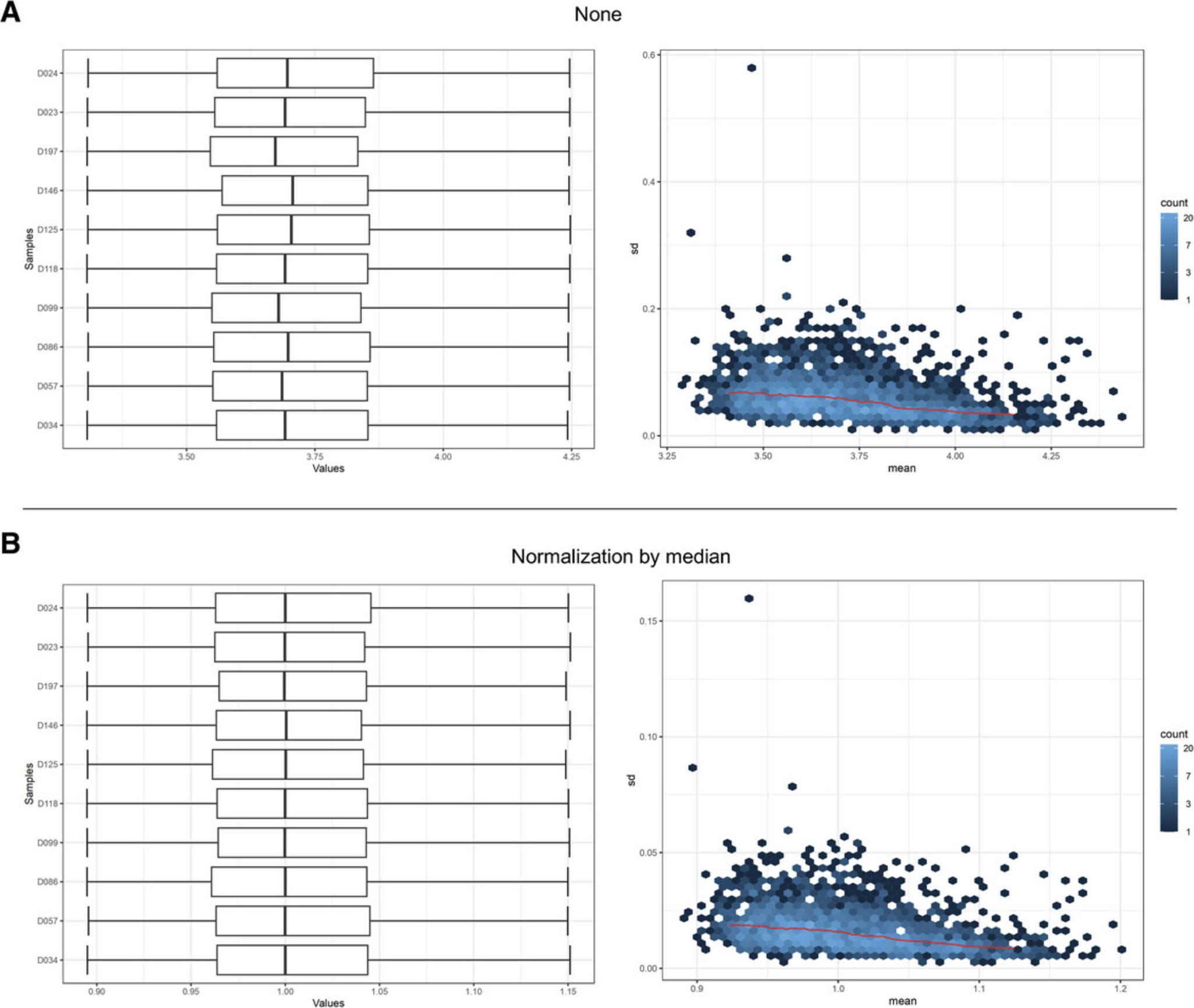
15.Select “Normalization by median” and click “Submit.”
16.Click the “Downloads” link on the upper navigation tracker. Stay on the “Files & Scripts” tab and download the “data_normalized.csv” file.
Basic Protocol 7: PREPARING MULTIPLE GENE EXPRESSION TABLES FOR META-ANALYSIS
As the cost of collecting transcriptomics data decreases and public data repositories grow quickly, it has become much easier these days to find multiple datasets testing the same hypothesis. The statistical power of individual transcriptomics DEA is quite low for most DEGs. In addition, analysis results are sensitive to even moderate outliers, which can greatly increase the number of false positives and false negatives. Meta-analysis can help overcome this issue by integrating results across multiple independent datasets to prioritize genes with consistent evidence for differential expression. In this protocol, we introduce how to use ExpressAnalyst for initial processing of multiple expression tables in preparation for the statistical and functional meta-analysis.
This protocol uses three datasets on helminth infections. Helminths are parasitic worms that impact ∼2 billion people worldwide (Oyesola & Souza, 2022). Here, we analyze three published microarray gene expression datasets of the liver tissue from both infected and control mice (Zhou et al., 2016).
Necessary Resources
Hardware
- A computer with internet access
Software
- An up-to-date web browser such as Google Chrome, Mozilla Firefox, or Safari, with JavaScript enabled (see Internet Resources)
Files
- None
1.Go to the ExpressAnalyst home page and click “Start Here” to access the module overview. Find the “Statistical & Functional Analysis” section and click the “Start Here” button located underneath the multiple gene expression table input type.
2.Click “Try Examples.” Clicking “Yes” will upload and process all three tables. However, we want to demonstrate these steps, so download and save each of the files. Open each of the three files and examine its content. All datasets must be from the same species and must be described by the same metadata labels, otherwise it will not be possible to compare results.
3.Click the “Data Upload” icon at the top of the page and choose the three files that you just downloaded. Click “Upload” and then “Done!”
4.We first need to perform annotation, missing value estimation, filtering, and normalization for each of the three uploaded datasets. In the “Data annotation” section, set the data value type to “Normalized values,” set the data type to “Microarray data (intensities),” set the organism to mouse, and the ID type to “Entrez ID” (Fig. 36). Click “Submit.”
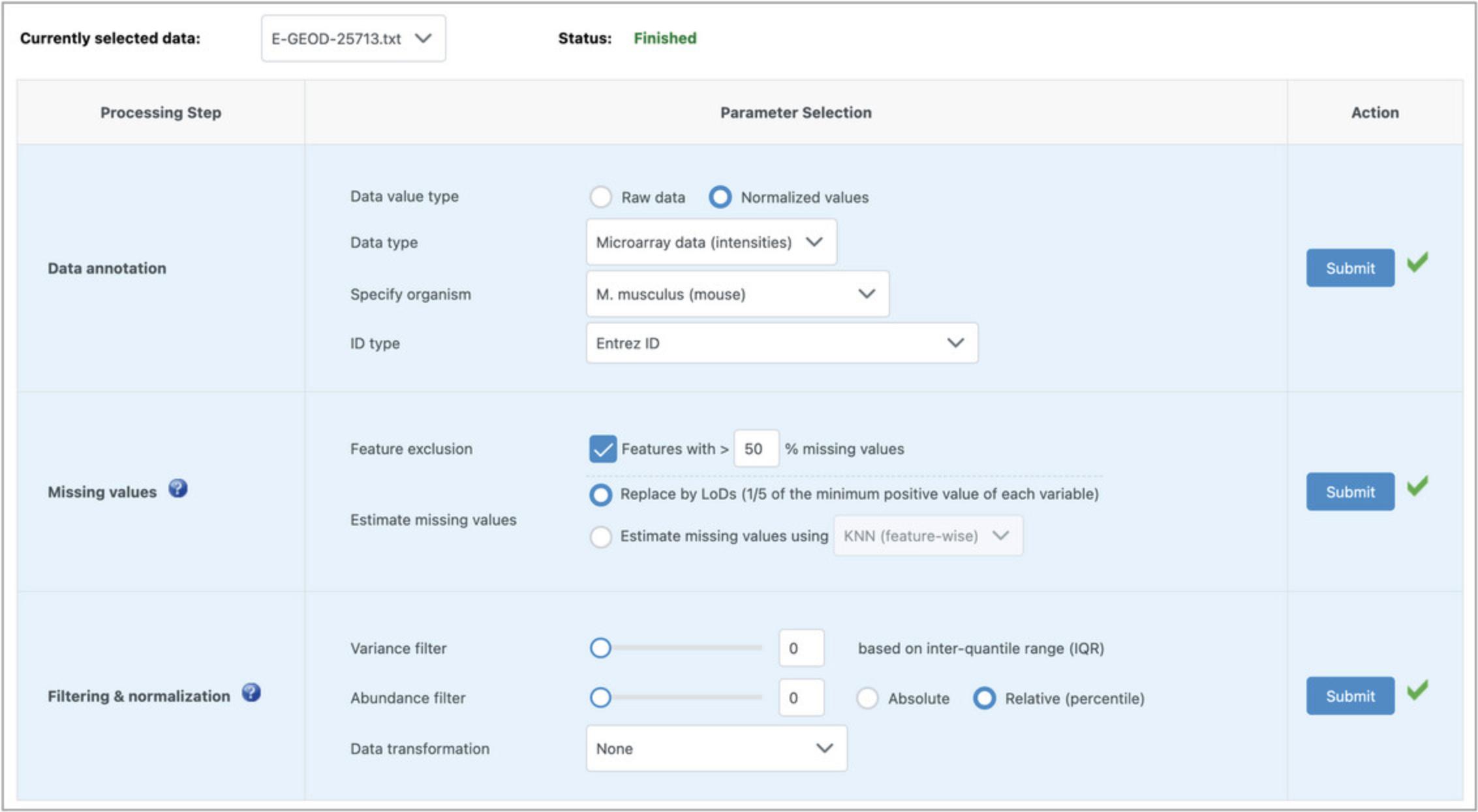
5.This dataset has no missing values, so it does not matter what the parameters are for the “Missing values” section. Leave the defaults and click “Submit.”
6.These datasets are already filtered and normalized, so in the “Filtering & normalization” section, set both the variance and abundance filters to 0 and leave “None” for the data transformation. Click “Submit.” Now the data status above the data processing table should have changed from “Incomplete” to “Finished.”
7.Find the dropdown menu above the data processing table and change the “Currently selected data” to the second dataset. Notice how this dataset has an “Incomplete” status. Repeat steps 4 to 6 for the second dataset, then select the third dataset and repeat steps 4 to 6 again. Click “Proceed.”
8.A dialog will pop up telling us that the data passed the integrity check. Click “Next” to proceed to the “Data Quality Check” page.
9.There is a clear batch effect with a strong pattern of separation according to technical platforms along PC1, so we will use ComBat for batch effect correction (Johnson et al., 2007). Check the box next to “Adjust study batch effect (Combat)” and then click “Update” (Fig. 37).

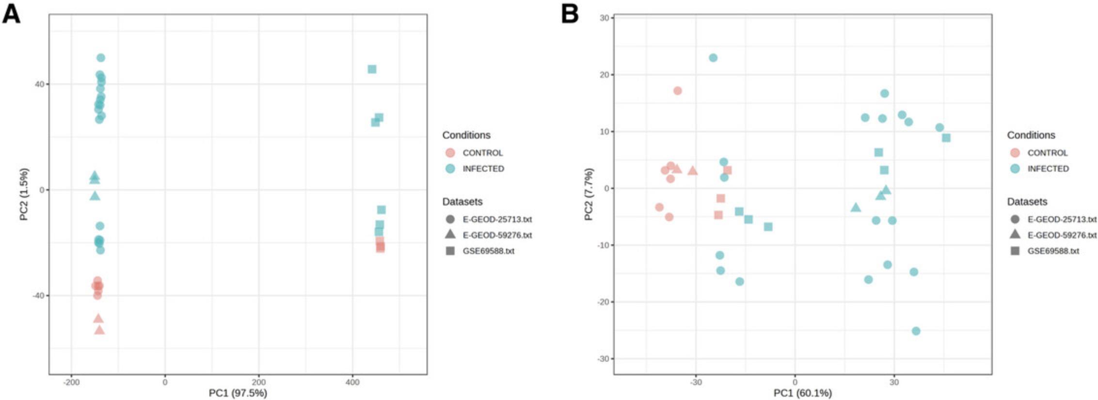
10.We have now finished the data processing for meta-analysis. Click “Proceed” to move to the statistical and functional analysis, which will be covered in Basic Protocol 8.
Basic Protocol 8: STATISTICAL AND FUNCTIONAL META-ANALYSIS OF GENE EXPRESSION DATA
The objective of meta-analysis is to identify genes that are consistently dysregulated across multiple datasets (Xia et al., 2013). There are two general approaches for this: 1) to directly merge the datasets and then perform a single DEA of the merged data, or 2) to perform DEA on each dataset separately and then combine their summary statistics (i.e., p -values or effect sizes). ExpressAnalyst supports both approaches, although in general we do not recommend direct merging unless the datasets are very similar e.g., all measured using the same platform and protocol. After statistical analysis, functional analysis can be performed on the list of DEGs identified during meta-analysis using the same set of visual analytics tools introduced in Basic Protocols 3 to 5, plus an additional tool specifically for comparing results across multiple datasets. Here, we continue analyzing the processed data from Basic Protocol 7 to perform statistical and functional meta-analysis.
Necessary Resources
Hardware
- A computer with internet access
Software
- An up-to-date web browser such as Google Chrome, Mozilla Firefox, or Safari, with JavaScript enabled (see Internet Resources)
Files
- None
1.This protocol requires Basic Protocol 7 for meta-analysis data processing and normalization. If you have not just completed Basic Protocol 7, please do so. You should be on the “Identifying significant features with complex metadata” page to begin this protocol. Make sure that “Control” is chosen as reference group and change “Contrast” to “Infected” and leave the rest as default. Click “Submit.”
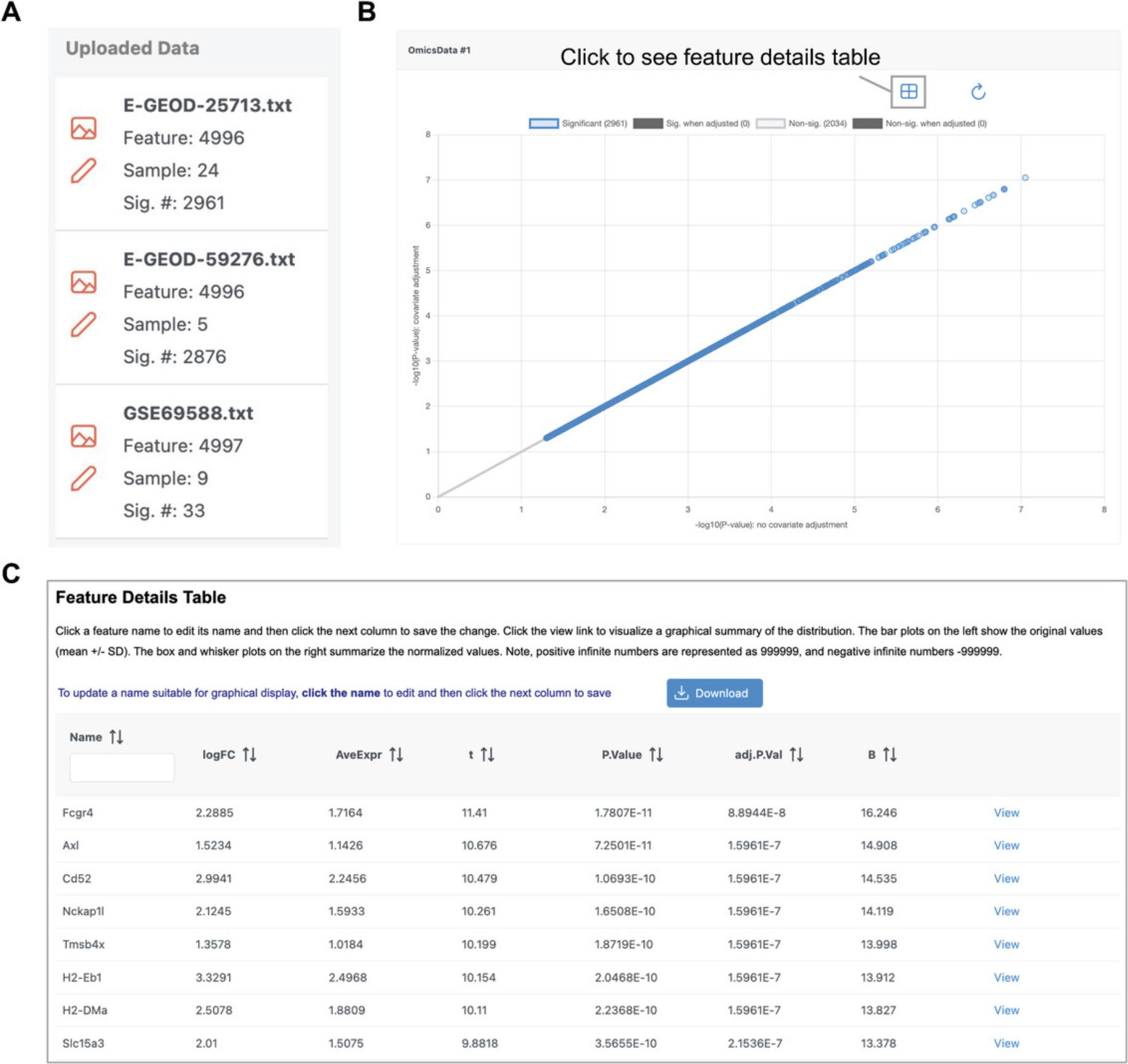
2.A graphical summary of the results is generated for each dataset. Scroll down to the “Omics Data #1” panel and click one of the points to view the corresponding feature plot (Fig. 39B). Click the table icon in the top right of the “Omics Data #1” panel to view a table of the summary statistics (Fig. 39C). Once you have finished examining the results, click “Proceed.”
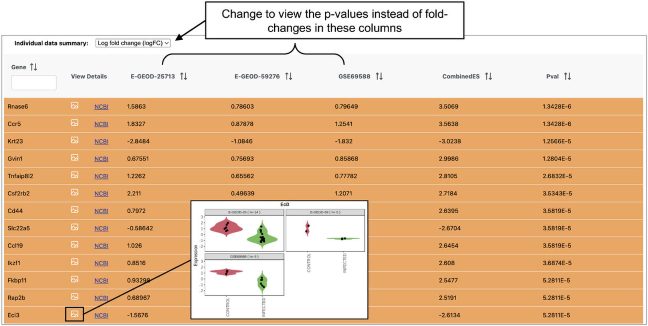
3.The next step is to integrate the DEA results across datasets. Look over all the integration strategies. Go to the first method (“Combining P -values”), leave the method as “Fisher's method,” and click “Submit” and then “Proceed.”
4.Click “Previous” to go back to the meta-analysis page. Go to the second strategy (“Combining Effect Sizes”). There are two different methods for performing this integration, using a “Fixed Effects Model,” or using a “Random Effects Model.” Click the “Cochran's Q-Test” button.
5.Select “Random Effects Model” from the dropdown menu in the “Combining Effect Sizes” section. Leave the p -value threshold as 0.05.Click “Submit” and “Proceed.”
6.There are 1703 significant results, a good number for visualization and functional analysis. Click “Proceed.”
7.The analysis overview has the same tools that were introduced in Basic Protocols 3 and 4.Click “Enrichment Network.” In the pop-up, leave “Meta-analysis results” selected and click “Proceed.”
8.In the “Enrichment Analysis” pane, change the “Type” to “GSEA” and click “Submit.” There are many significant results, and the labels are all overlapping and difficult to read. Find the horizontal toolbar and change the “Node” dropdown to “Label.” Go to the “Display” tab in the “Node Label Customization” dialog, change the dropdown to “Unlabel all nodes” and click “Submit” (Fig. 41).
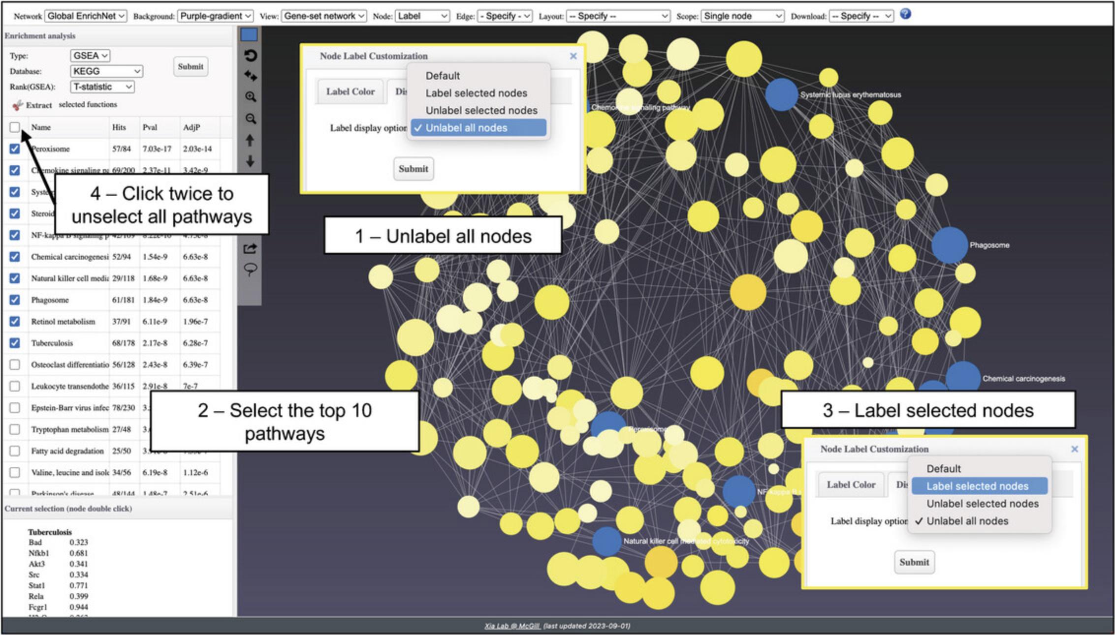
9.Go to the results table. Select the top 10 most significant pathways. Change “Label” to unspecified and then back to “Label” to access the pop-up again. Change the dropdown to “Label selected nodes” and click “Submit.” You will see that all the selected nodes are now labeled. However, these nodes are colored with the same highlight color. To restore their default color styles based on expression profiles, go to the results table, check, and then immediately uncheck the “Select all” box to remove all the checked boxes (Fig. 41).
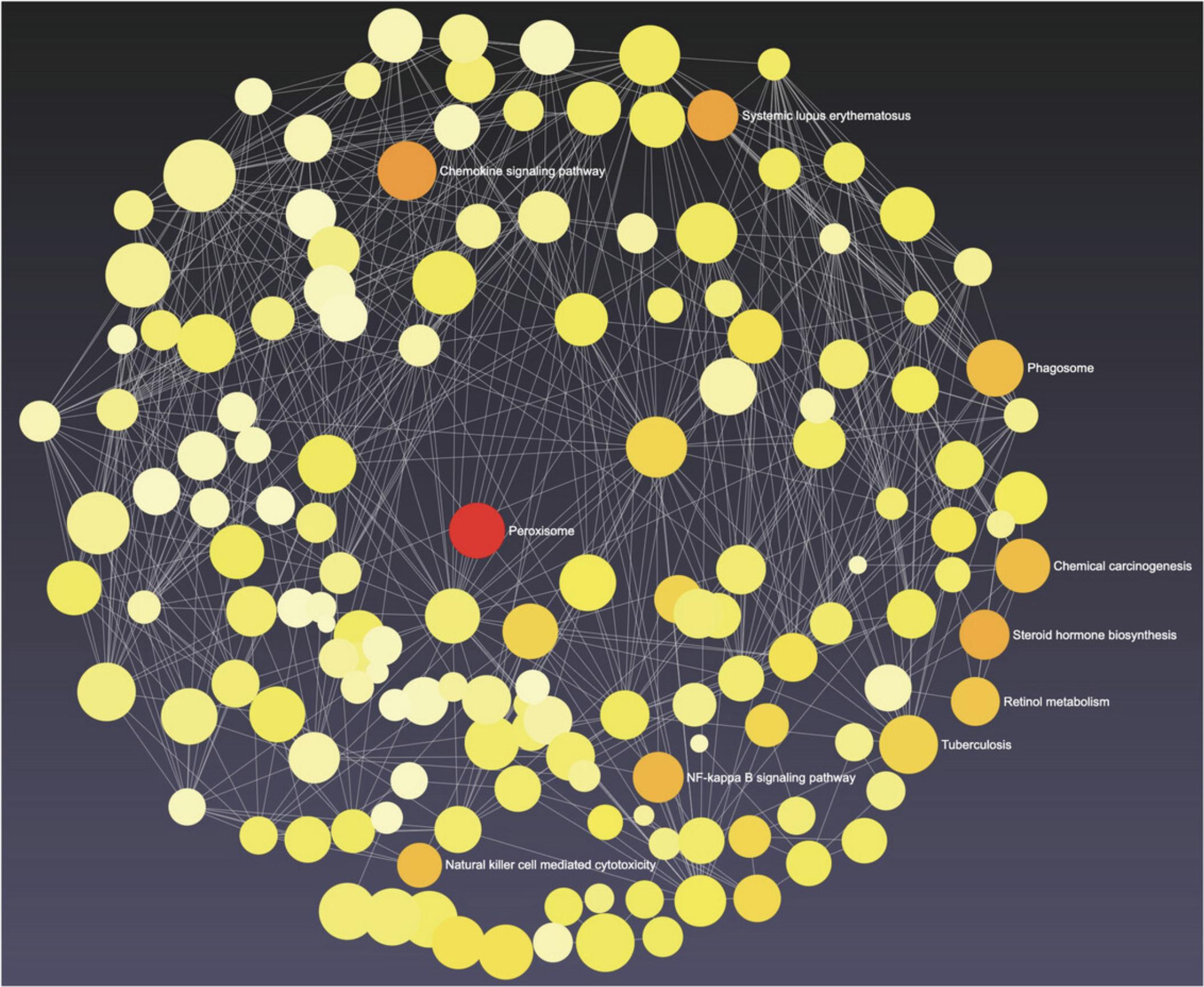
10.The network is now much more interpretable and easier to read, with only the key nodes labeled. Some of the labels are still overlapped by other nodes. Click and drag individual nodes until every label is visible (Fig. 42).
11.Navigate back to the “Analysis Overview” and click the “Upset Diagram” button. Keep the defaults: all three datasets included but leave the “Meta-analysis features” unchecked. Click “OK.”
12.The diagram allows us to explore DEG overlap across datasets (Fig. 43). Hover your mouse over any bar to see how many of those genes are present in the other interactions.
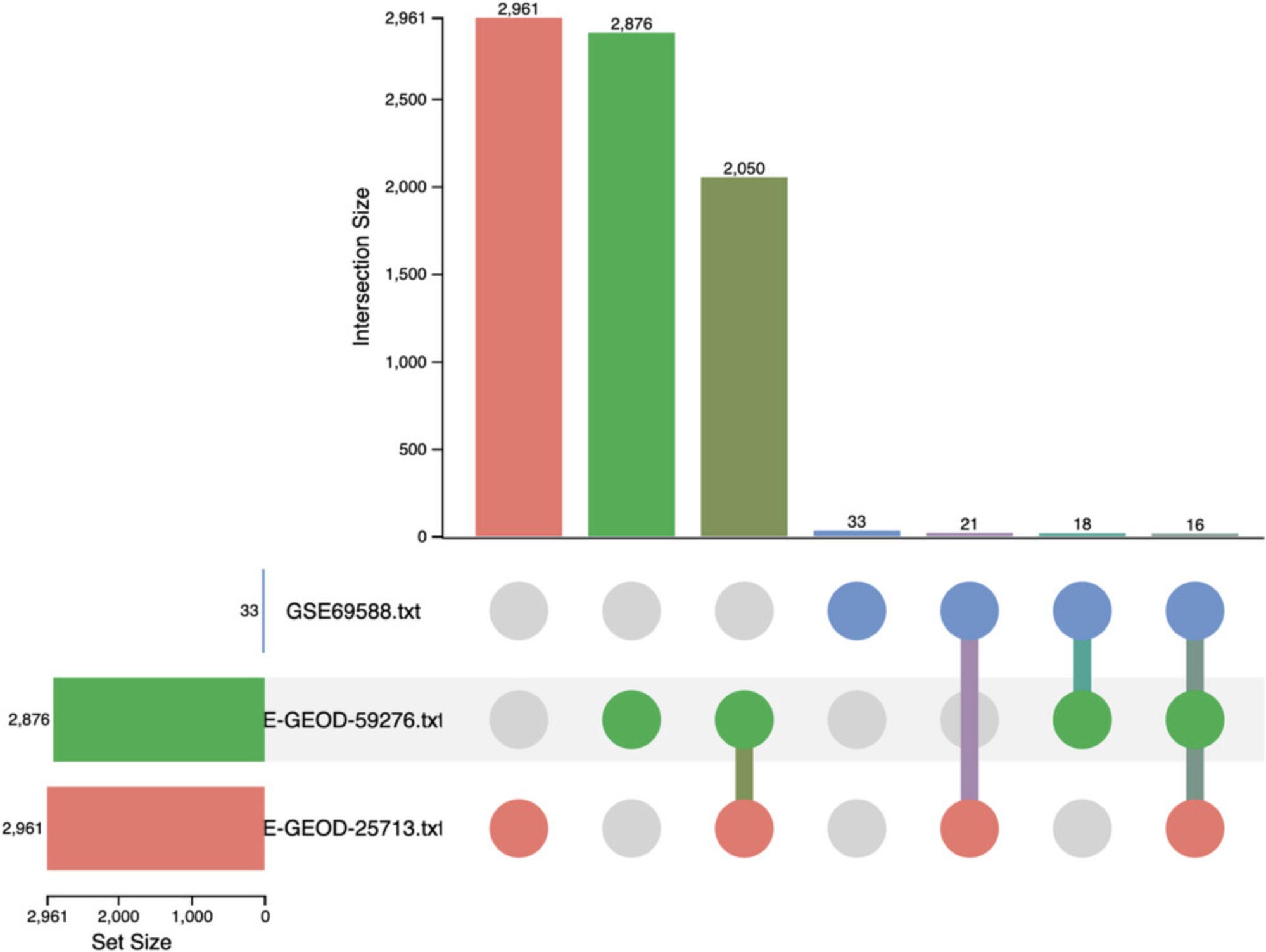
13.Click the last column of dots corresponding to the DEGs that were present in all datasets. This will display the gene names in the bottom left “Feature Members” panel. Now go to the “Enrichment Analysis” panel and click “Submit.” This will perform ORA with the KEGG database using the genes in the “Feature Members” panel.
14.Go to the navigation bar at the very top of the page and click the “Downloads” link to view and download the results.
Basic Protocol 9: FUNCTIONAL ANALYSIS OF TRANSCRIPTOMICS SIGNATURES
Differential expression analysis (DEA) produces lists of differentially expressed genes or proteins, also known as transcriptomic or proteomic signatures. These lists can be saved, and then uploaded to ExpressAnalyst directly through the list upload in the “Statistical and Functional Analysis” module. DEA results are also commonly available as supplementary files in the published literature, providing another source of transcriptomic signatures. Since the data are small relative to an omics data table, we can easily upload multiple lists simultaneously to visually compare them. We can also perform functional analysis on the list of uploaded genes. In this protocol we introduce the different list formats that are accepted by ExpressAnalyst, and then demonstrate how to compare multiple uploaded lists with a heatmap.
Necessary Resources
Hardware
- A computer with internet access
Software
- An up-to-date web browser such as Google Chrome, Mozilla Firefox, or Safari, with JavaScript enabled (see Internet Resources)
Files
- None
1.Go to the ExpressAnalyst home page and click “Start Here” to view the module overview. Find the “Statistical & Functional Analysis” section and click the “Start Here” button underneath the list input type.
2.Go to “Try Examples,” keep “Gene list 1” selected, and click “Submit.” This will populate the data input with a list of IDs, along with the appropriate species and ID type.
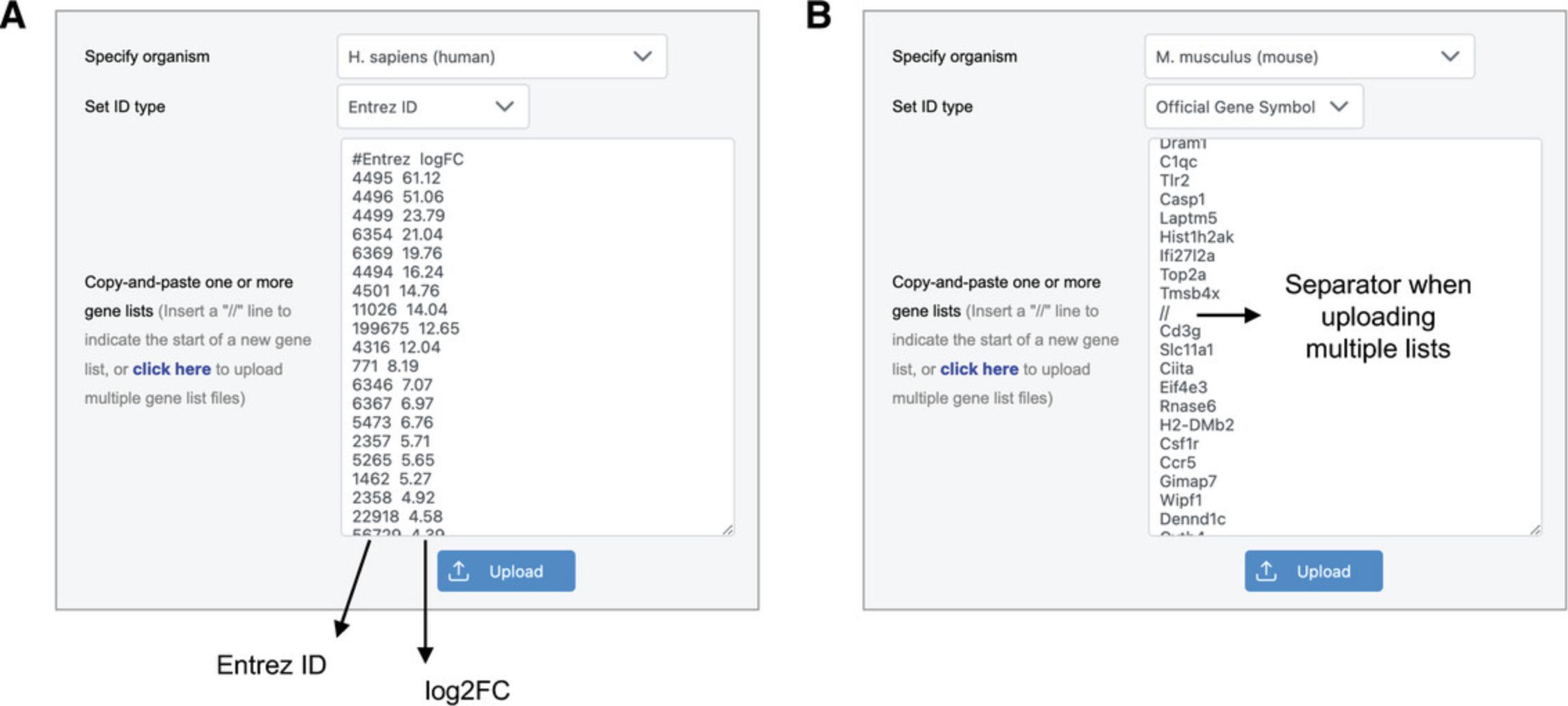
3.Click “Try Examples” again, select the last example data called “Multiple Lists,” and click “Submit.”
4.Click the “Upload” button beneath the text input area, and then click “Proceed.”
5.Find the heatmap icon and click the “ORA” button. This will show a new type of heatmap, designed to compare multiple lists (Fig. 45).
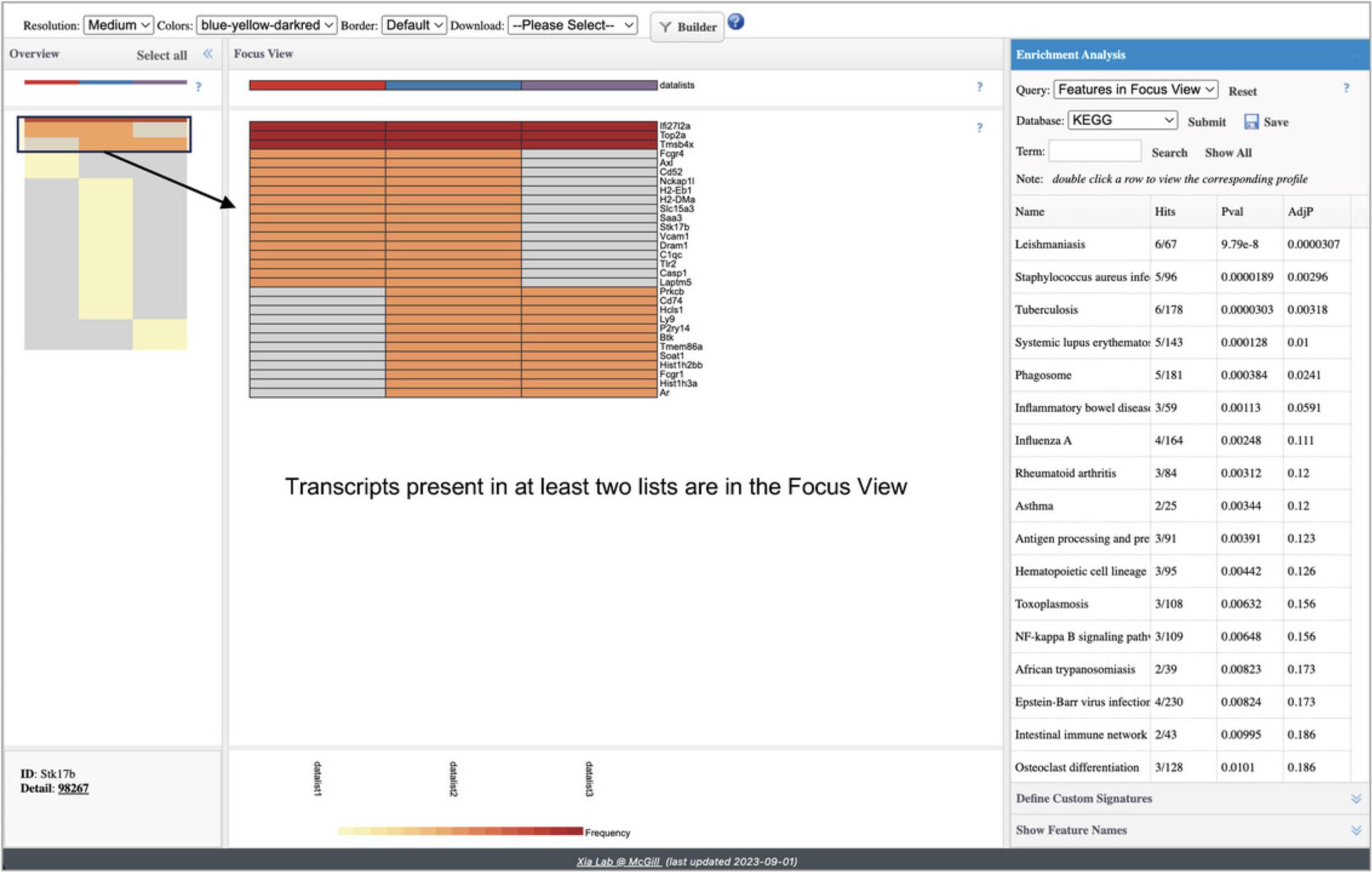
6.In the “Overview” panel on the left, use your mouse to drag-and-select the rows containing red and orange cells. Those selected rows will show in the “Focus View.” Then, go to the “Enrichment Analysis” panel on the right and click “Submit.”
7.Navigate back to the “Analysis Overview,” find the network icon and click the “Enrichment Network” button. A dialog with a dropdown will appear. We have the option of choosing one of the three uploaded lists; leave “datalist 1” selected and click “Proceed.”
8.Click the “Downloads” button to view all the results from this protocol.
Basic Protocol 10: DOSE-RESPONSE AND TIME-SERIES DATA ANALYSIS
As the cost of acquiring transcriptomics datasets decreases over time, we see more datasets that measure groups of samples along a continuous dimension, such as chemical doses or time points. A statistical method called “dose-response analysis” was developed by the field of toxicology to identify the concentration at which a biological assay responds to chemical exposure (Thomas et al., 2013). Dose-response experimental designs typically include a control group (dose = 0) and at least four different dose groups, typically with the same number of replicates in each group. To perform transcriptomics dose-response analysis, the data are processed and normalized according to standard protocols, and then differential analysis is used to identify genes that have a relationship with dose. All genes that pass the DEA filters are used for dose-response curve fitting, in which a suite of linear and non-linear curves is fitted to the expression of each gene, and the best fit model for each gene is kept. Next, the curve is analyzed to determine the precise concentration at which the fitted curve departs from the expression values in the control group (called the gene benchmark dose, or BMD). The collection of gene BMDs can then be analyzed at the pathway or whole-transcriptome level to determine the concentration at which specific pathways respond, or the concentration at which we observe a robust transcriptomic response. ExpressAnalyst uses the FastBMD implementation of dose-response analysis (Ewald et al., 2021).
While this method was developed for analyzing dose-series data in a toxicology context (National Toxicology Program, 2018), the same statistical approach can be used to analyze data measured along any continuous gradient, for example time-series or even temperature. In this protocol, we introduce BMD analysis with a chemical exposure dataset. Rats were exposed to five concentrations of bromobenzene for 2 weeks, at which point transcriptomic data were measured with microarrays in liver tissue (Thomas et al., 2013).
Necessary Resources
Hardware
- A computer with internet access
Software
- An up-to-date web browser such as Google Chrome, Mozilla Firefox, or Safari, with JavaScript enabled (see Internet Resources)
Files
- None
1.Go to the ExpressAnalyst home page and click “Start Here” to view the module overview. Find the “Statistical & Functional Analysis” section and click the “Start Here” button that is underneath the single table input type.
2.Go to “Try Examples” and select the “Bromobenzene” example data. Click “Submit” and then “Proceed.”
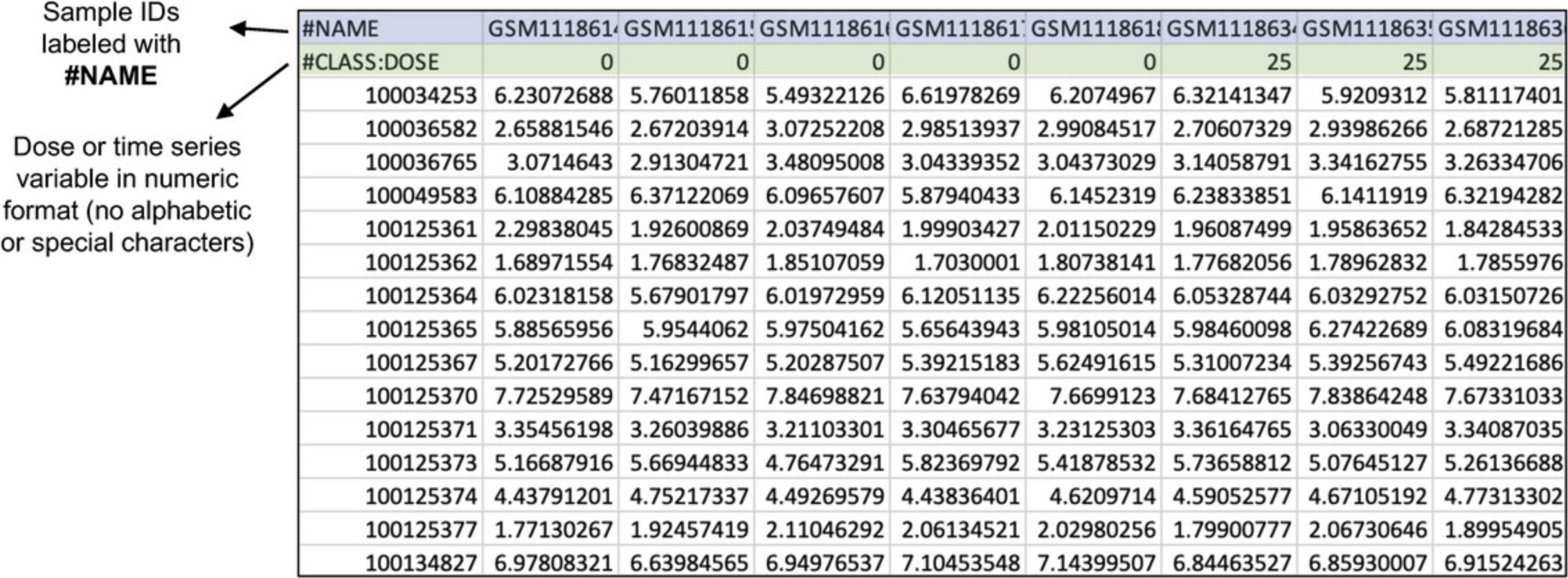
3.The “Omics data overview” shows that there is a control group (dose = 0) and five dose groups (doses = 25, 100, 200, 300, and 400). When you are done viewing the data, click “Proceed.”
4.This dataset was already normalized. Leave the filtering defaults, select “None” for normalization, and click “Submit.” When you are done viewing the PCA and box plots, click “Proceed.”
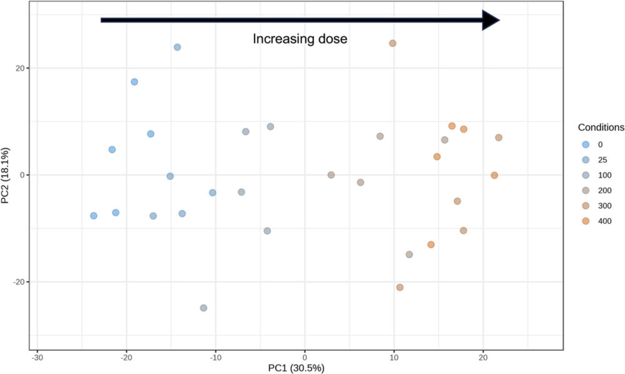
5.In dose-response analysis, DEA is a pre-filtering step, used to remove genes that do not change over the measured conditions prior to the computationally intensive curve fitting step according to a standard design, hence the interface is greatly simplified. Make sure that “DOSE” is selected as the dose/time factor and that “0” is selected as the control condition. Leave the “Statistical method” as “Limma.” Click “Submit” and then “Proceed.”
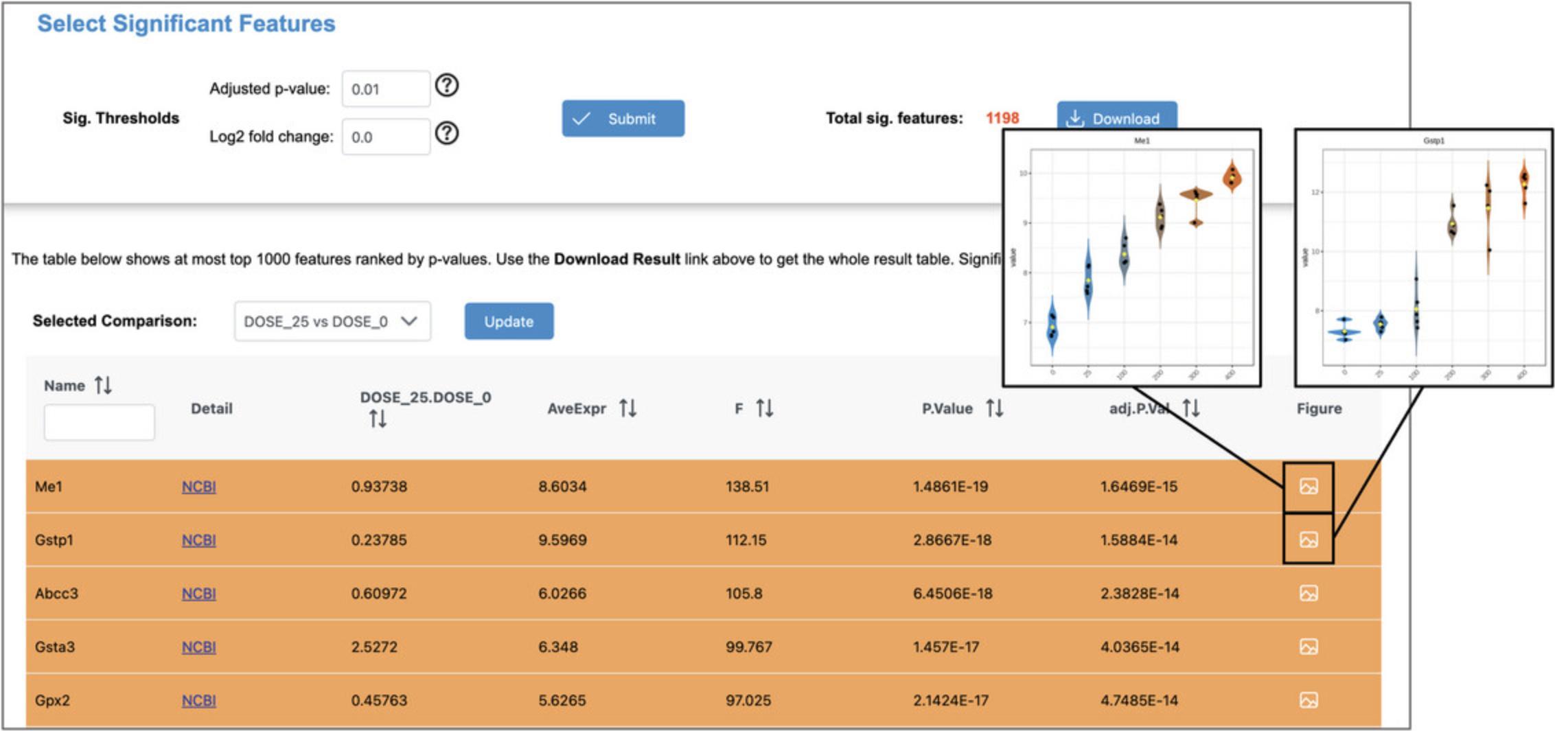
6.There should be 2018 significant features. Change the “Adjusted p -value” from 0.05 to 0.01 and click “Submit” to update to 1198 significant features. Click the “Graphical Summary” to view feature plots of the top few rows (Fig. 48). Change the “Selected Comparison” dropdown to DOSE_300 vs. DOSE_0. You should see that the log2FC column changed, but that the p -values stayed the same. Click “Proceed.”
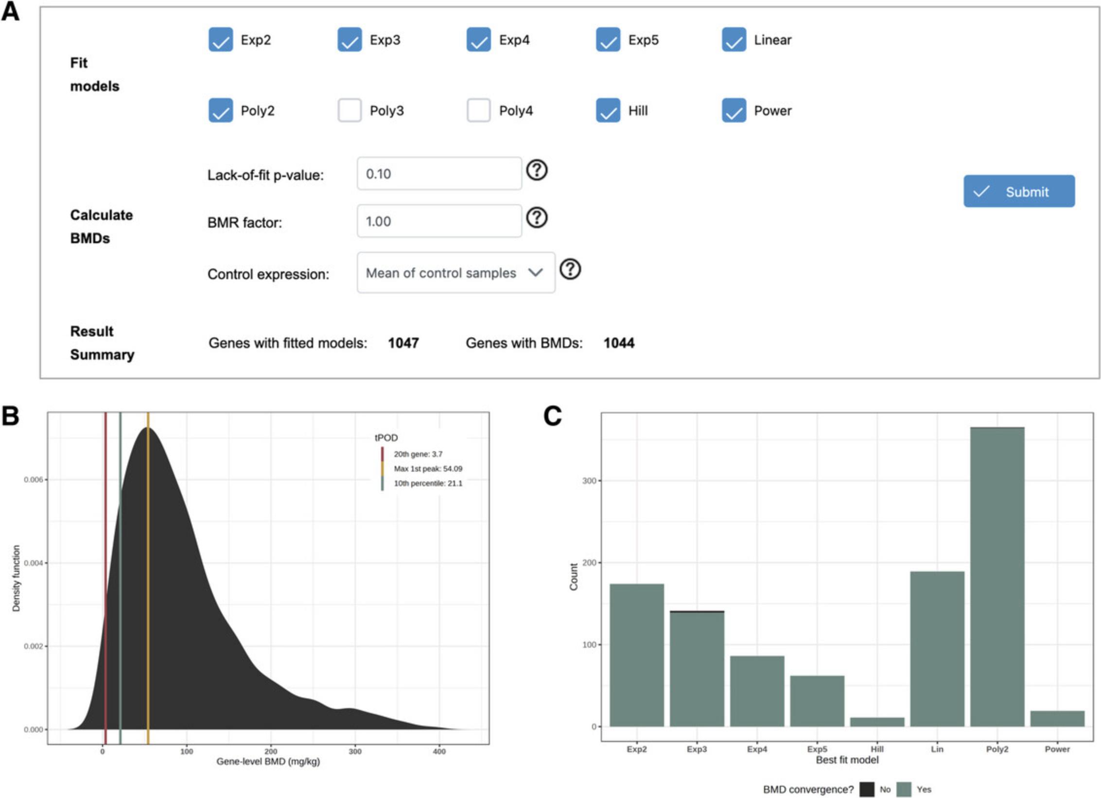
7.Leave the defaults (Fig. 49A) and click “Submit.” This is quite computationally intensive, hence this step could take several minutes to complete.
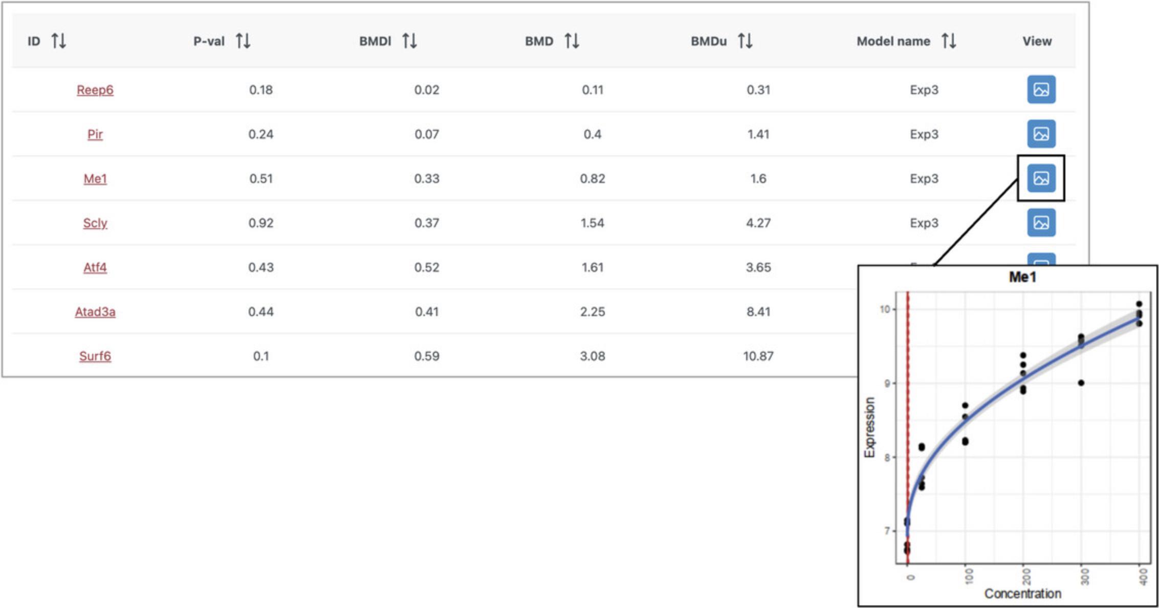
8.Navigate to the results table and click the button in the “View” column for several of the genes.
9.Click “Proceed” to go to the “Analysis Overview.” Click the “Accumulation Plot” button.
10.By default, pathway analysis was performed with the KEGG database.
11.There is one pathway with a very high number of hits (“Metabolic pathways”) that makes it difficult to see the differences between the other pathways. Click the “Metabolic pathway” row in the results table to remove it from the plot. Now the other pathways become easier to see (Fig. 51).
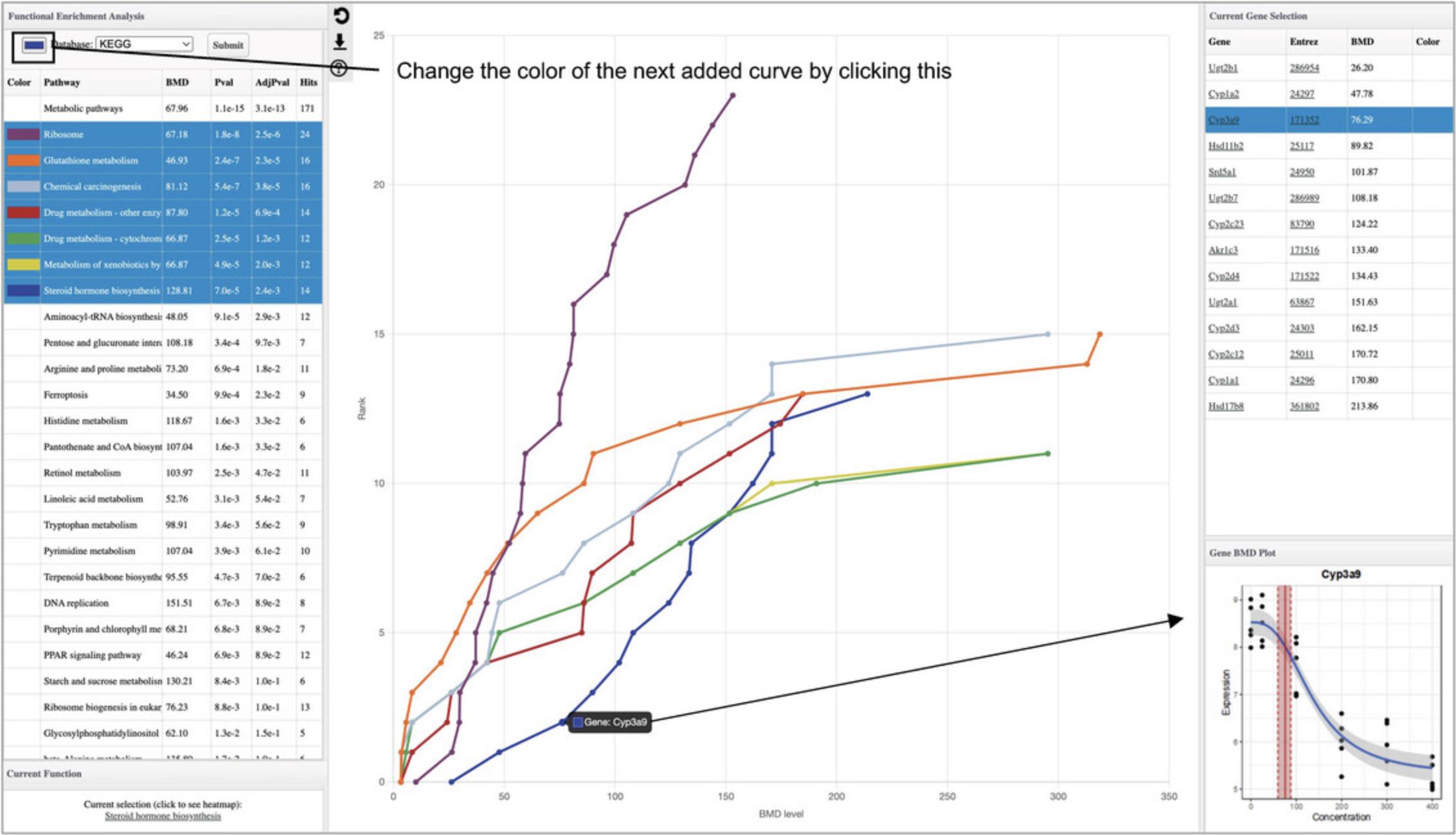
12.Click the colored box next to the “Database” label in the top left (Fig. 51) and choose a new color. Next, click the next most significant pathway that is not highlighted to add an accumulation plot for that pathway in the selected color. Repeat these two steps to add a few more pathways to the diagram.
13.Click the underlined pathway name in the “Current Function” panel (below the enrichment result table) to generate a heatmap summarizing all fitted curves within that pathway. Hover your mouse over a point in the accumulation plot and click to view the fitted curve for that gene.
14.Click the “Downloads” link on the top navigation tracker to view and download all the results generated during the analysis session.
Basic Protocol 11: RNA-seq READS PROCESSING AND QUANTIFICATION WITH AND WITHOUT REFERENCE TRANSCRIPTOMES
The first step in an RNA-seq analysis starts with quantification of the raw reads from FASTQ files. This involves performing quality control, trimming low-quality reads, and aligning cleaned reads to a reference genome or transcriptome (Conesa et al., 2016). This is the most computationally intensive part of a basic RNA-seq analysis pipeline, and ExpressAnalyst provides two options: users may upload compressed FASTQ files (.fastq.gz) to the ExpressAnalyst server for remote processing, or they may install the ExpressAnalyst stand-alone (ExpressAnalystSA) Docker for local processing (Liu et al., 2023). When using the remote option, data upload is limited to four concurrent users, users are limited to a maximum of 4-hr upload session, and each user may only store and process 30 GB of FASTQ files at one time. In contrast, the local option allows users to avoid the time-consuming data upload step and does not impose any limitation on the dataset size, although it is slightly more complicated to set up for the first time.
In this protocol, we guide users through installing the ExpressAnalystSA Docker and performing RNA-seq reads quantification with kallisto and Seq2Fun (Bray et al., 2016; Liu et al., 2021). Downstream statistical and functional analysis are covered in Basic Protocols 2 to 5.Note that if users do not envision performing raw data processing and are primarily interested in analyses beginning with a count table, they can skip this protocol and proceed directly to Basic Protocol 2.
Necessary Resources
Hardware
- A computer with internet access, equipped with Intel or AMD CPU, and at least 16 GB RAM and 250 GB free storage
Software
- An up-to-date web browser such as Google Chrome, Mozilla Firefox, or Safari, with JavaScript enabled (see Internet Resources)
Docker Desktop (see Internet Resources)
Files
- None
1.Go to the ExpressAnalyst homepage and click on the “Tutorials” tab. Click the download link for “Basic Protocol 11 (FASTQ files).” This will navigate to the Xia Lab file server, which hosts large datasets and databases for download. Click “Download.”
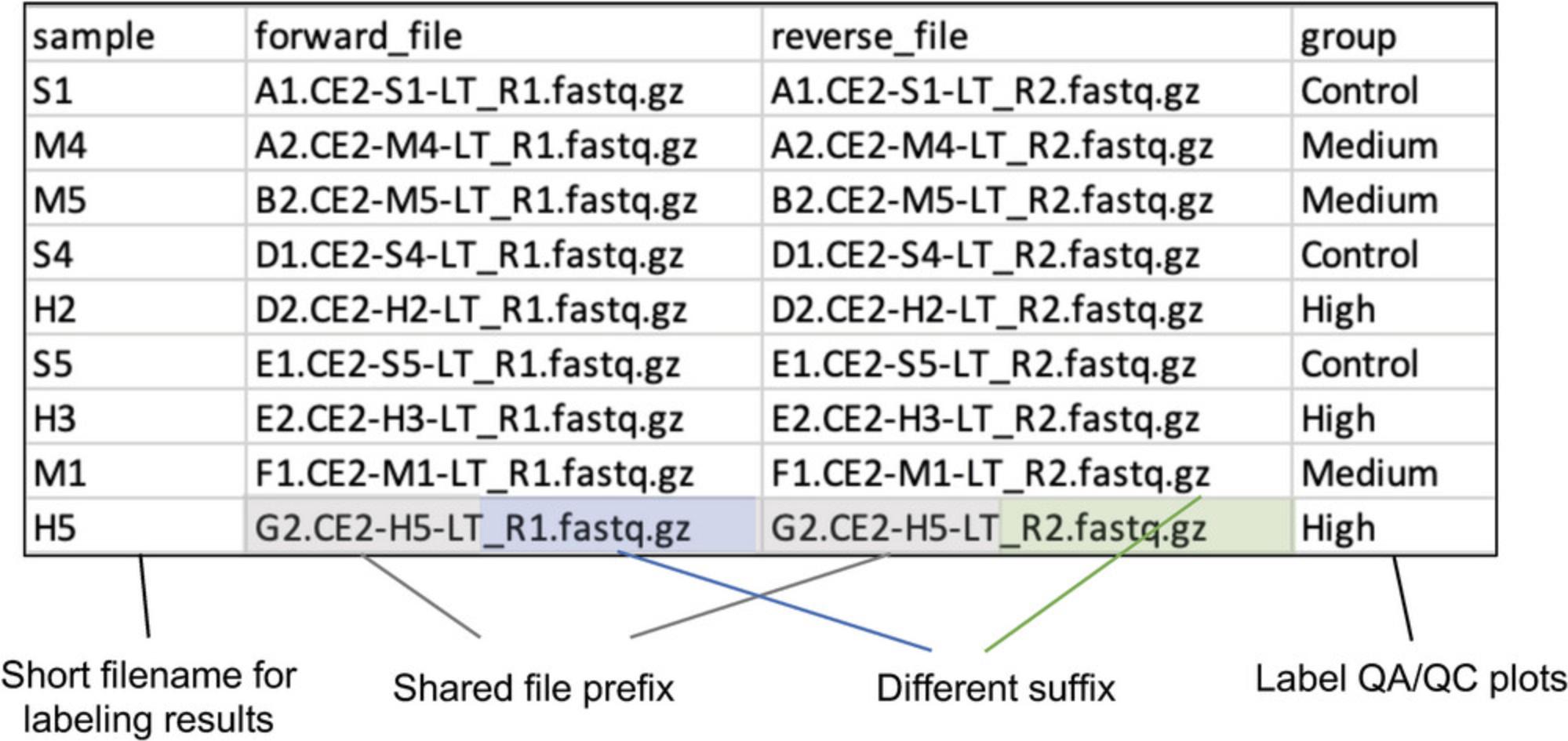
2.Expand the zipped file. Inside there should be 18 FASTQ files and a “metadata.txt” file. Right-click the “metadata.txt” file and open it with a spreadsheet program like Microsoft Excel.
3.Start the Docker software on your computer. If you are using Docker Desktop, click the Docker icon and wait while the software initializes. You can tell that Docker Desktop is running if the Docker Desktop window shows an overview of your Docker containers, or if you click the small Docker icon (next to where the Wi-Fi connection status is shown) and the dropdown menu says, “Docker Desktop is running.” We do not include screenshots here because Docker Desktop looks different for different operating systems.
4.To download the most recent version of the ExpressAnalystSA Docker image to your computer, open your command line, copy-paste this text and hit enter:
- docker pull dockerxialab/expressanalyst_docker:latest
5.Determine your home directory. This can vary depending on your operating system.
6.Stay in the command line and enter the command:
- docker run -ti --rm -p 8080:8080 -v HOME_DIRECTORY:/data dockerxialab/expressanalyst_docker:latest
but replace the words HOME_DIRECTORY with the home directory that you determined in the previous step. For example, with a home directory of “/Users/jessica,” the complete command would be:
- docker run -ti --rm -p 8080:8080 -v /Users/jessica:/data dockerxialab/expressanalyst_docker:latest

7.Open a web browser (we recommend Chrome) and type localhost:8080/ExpressAnalystSA/ in the URL bar. You should see the ExpressAnalyst homepage. Click “Start Here.”
8.We need to first download the reference transcriptome and the ortholog database from the “Databases” page (https://www.expressanalyst.ca/ExpressAnalyst/docs/Databases.xhtml) (Fig. 54A). On the “With a Reference Transcriptome” tab, find the Gallus gallus (chicken) reference transcriptome and click the download icon (Fig. 54B). When the download link finishes loading, click the “Download” button. This file size is 644 MB.
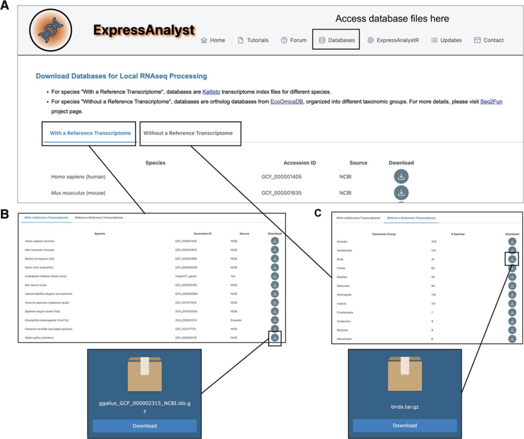
9.Navigate to the “Without a Reference Transcriptome,” find the “Birds” database, and click the download icon (Fig. 54C). When the download link finishes loading, click the “Download” button. The file size is 170 MB.
10.We will create a data directory for the analysis with a reference transcriptome. Create a folder called “Process_Kallisto.” Inside the folder, create three more folders: “DATABASE,” “FASTQ,” and “RESULTS.” Move the downloaded FASTQ files to the “FASTQ” folder and move the downloaded reference transcriptome to the “DATABASE” folder (Fig. 55).
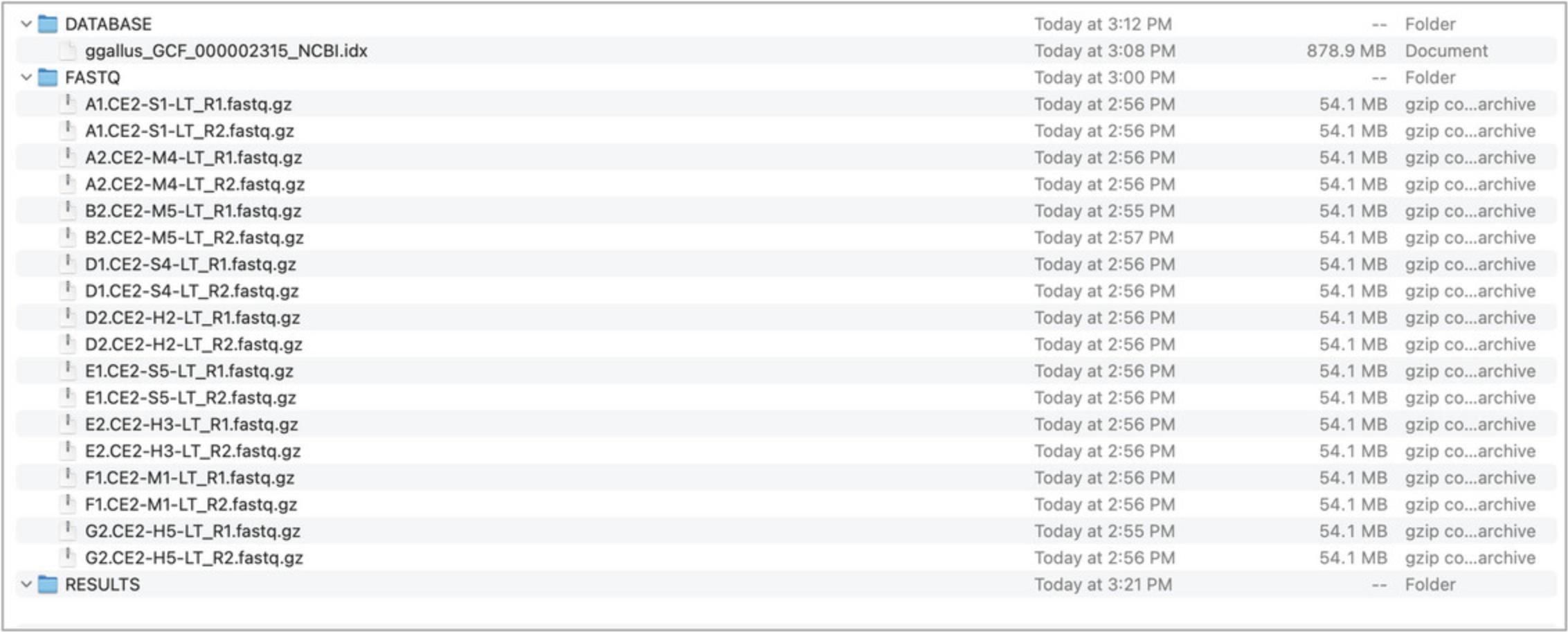
11.For Mac or Linux users, double-click the transcriptome file to decompress it (“.idx.gz” to “.idx”). When it is finished, delete the compressed transcriptome file to save space on your computer. If you are using a Windows computer and know how to use your command line to decompress “.gz” files you can do this, otherwise leave the file as is.
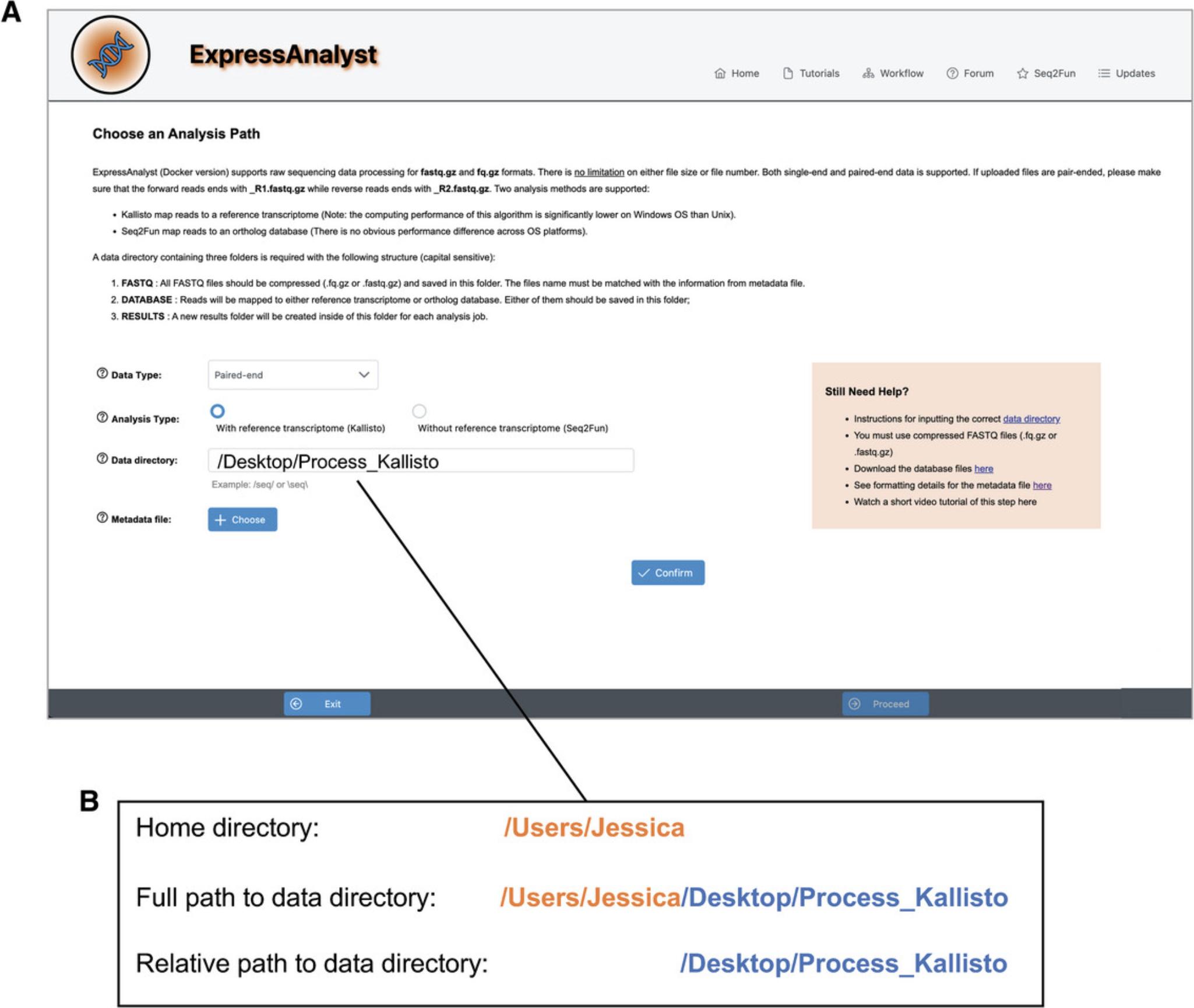
12.Go back to the browser tab where the ExpressAnalystSA Docker is running. Keep the “Data Type” as “Paired-end” and keep the “Analysis Type” as “With reference transcriptome (Kallisto).” Determine the relative path to your data directory (Fig. 56B), by considering the full path to your data directory and removing the home directory path that you used in the “docker run” command. Enter the relative path into the “Data directory” text input. Choose the “metadata.txt” file for the “Metadata file,” click “Submit,” and then click “Proceed.”
13.The Data Integrity Check page contains a summary of all the FASTQ files. Make sure that all files are there and properly labeled, then click “Proceed.”
14.Keep the “Minimum reads quality score” as 25.Find the number of cores on your computer. If you have >4, you can increase the number of cores to make the analysis run faster. It is also acceptable to leave this as 3.Click “Confirm,” click “Submit Job,” and then click “Confirm” in the dialog.
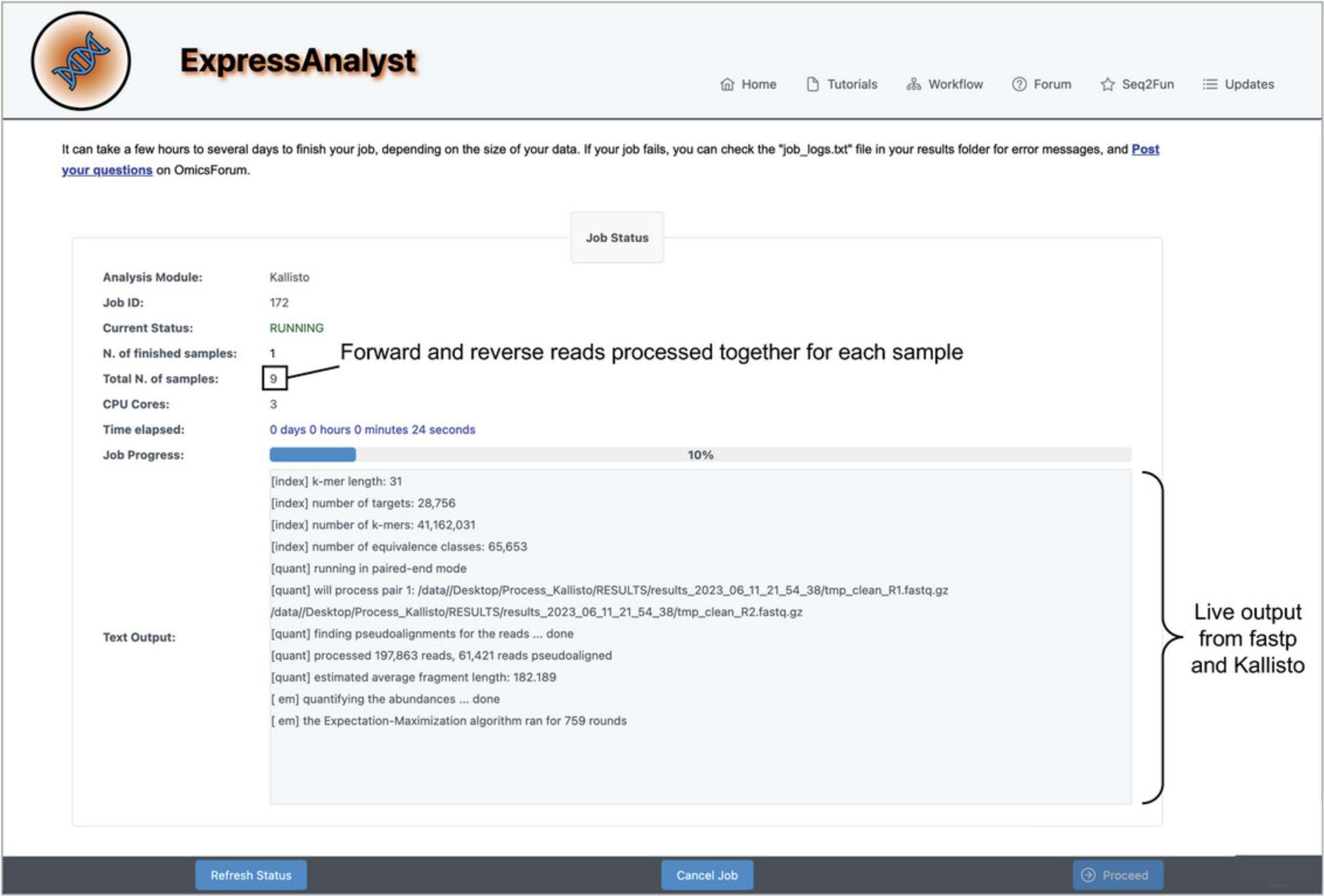
15.The processing job has started. Wait until the “Current Status” says “COMPLETE” instead of “RUNNING,” then click “Proceed.”
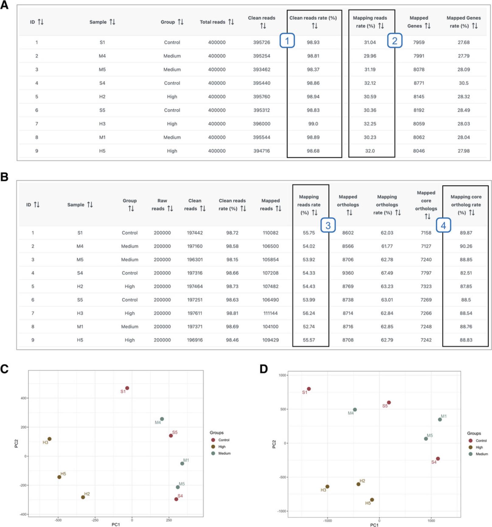
16.Click through the four different tabs to view the summary table and figures. When you are finished viewing the results, click “Download Results” in the bottom right.
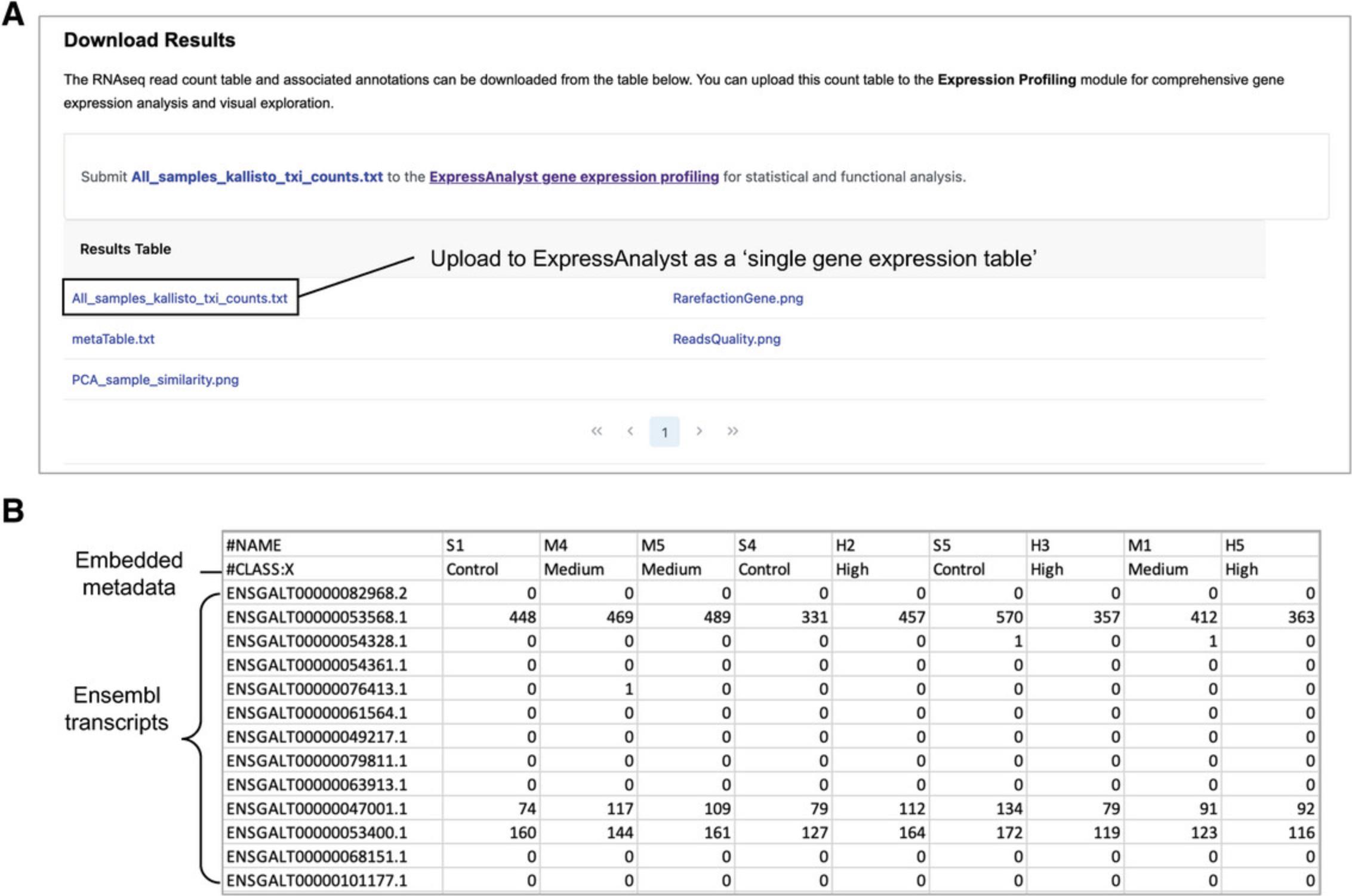
17.Download the “All_samples_kallisto_txi_counts.txt” file (Fig. 59A) and open it to view the format (Fig. 59B).
18.Navigate back to ExpressAnalyst home and click “Start here” to initiate a new analysis.
19.Create a new folder called “Process_Seq2Fun.” Inside the folder, create three more folders: “DATABASE,” “FASTQ,” and “RESULTS.” Drag the FASTQ files from the previous analysis into the new FASTQ directory. Drag the downloaded birds ortholog database into the DATABASE directory.
20.Decompress the database file. Move the “birds_annotation_v2.0.txt” and “birds_v2.0.fmi” files directly inside of the DATABASE folder in the data directory. Delete the empty ‘birds’ folder.
21.Select files, parameters, and initiate job. Change to “Without a reference transcriptome (Seq2Fun).” Use the same metadata table that you used for the kallisto analysis. Click “Confirm” and then “Proceed.”
22.View the “Data Integrity Check” table. It should look the same as for the kallisto workflow since we are using the same samples. Click “Proceed.”
23.Leave the first three parameters as the defaults. If you changed the CPU cores in the kallisto analysis, change the CPU cores input here as well. Click “Confirm,” “Submit Job,” and then “Confirm.”
24.Seq2Fun is now running. Wait until the job view summary says “COMPLETED” and that 9 out of 9 samples have been processed. Click “Proceed.”
25.View results and interpret Seq2Fun-specific QA/QC parameters. Click “Download Results.”
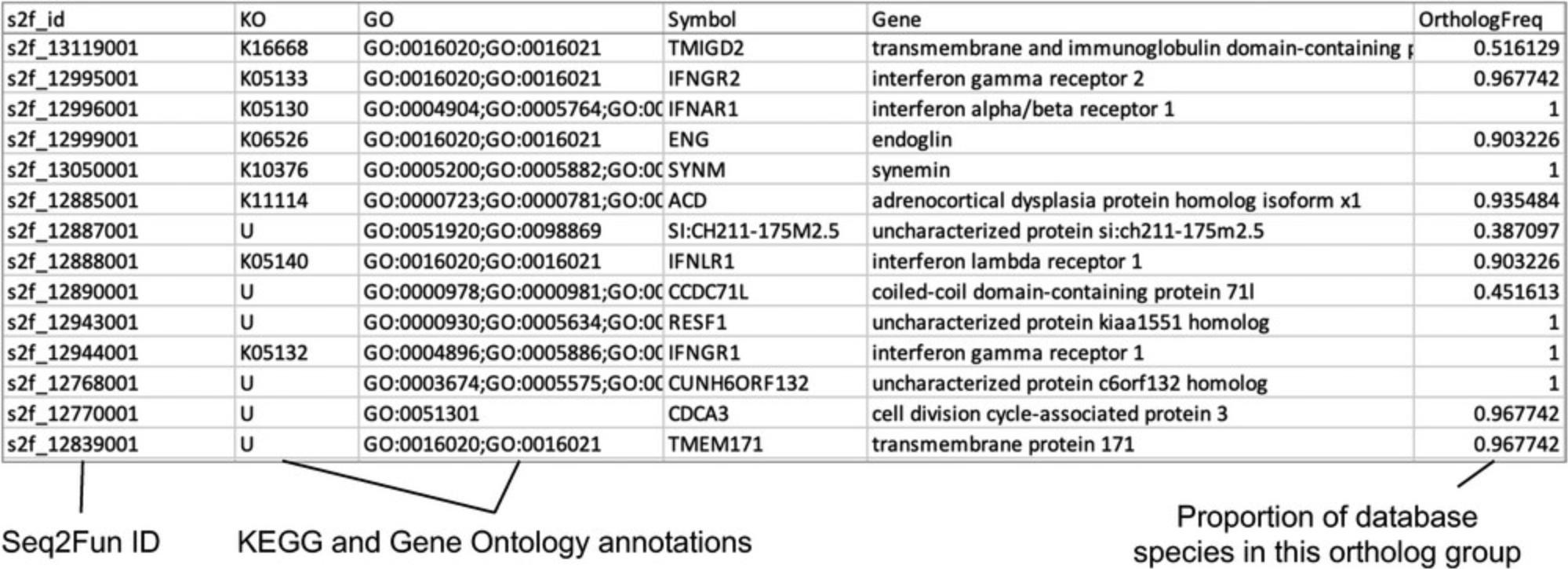
26.Download the “S2fid_abundance_table_all_samples_submit_2_expressanalyst.txt” file and open it to view. We see that the format is the same as the file generated by kallisto, except that the rows are now labeled with Seq2Fun ortholog IDs instead of with Ensembl chicken transcripts. Open the “S2fid_ortholog_annotation_all_samples.txt” file (Fig. 60).
COMMENTARY
Background Information
As sequencing and mass spectrometry technologies continue to improve, more researchers are collecting these datasets, and the average dataset size and complexity are increasing. ExpressAnalyst is part of the Analyst tool suite, a collection of web-based platforms that have been developed to allow researchers to easily analyze omics data through a user-friendly web interface, including MetaboAnalyst (metaboanalyst.ca) for metabolomics data analysis, NetworkAnalyst (networkanalyst.ca) for gene expression data analysis (before 2019), MicrobiomeAnalyst (microbiomeanalyst.ca) for microbiome data analysis, as well as OmicsAnalyst (omicsanalyst.ca) for multi-omics data integration (Lu et al., 2023; Pang et al., 2022; Zhou et al., 2021; Zhou et al., 2019). The core components of differential expression analysis and meta-analysis were previously published as NetworkAnalyst. In 2019, we decided to keep NetworkAnalyst as a dedicated platform for network analysis and visualization of gene lists, following the naming conventions with other network tools we developed for molecular signature analysis such as miRNet (mirnet.ca) for miRNA lists and OmicsNet (omicsnet.ca) for multi-omics lists (Chang et al., 2020; Zhou & Xia, 2018). The core gene expression profiling and meta-analysis components were separated out to form a new platform, ExpressAnalyst, dedicated for transcriptomics and proteomics data profiling. The split allowed us to efficiently build out ExpressAnalyst to support more data formats, including raw data processing, and more complex experimental designs (Liu et al., 2023). It would become too cumbersome to develop and overwhelming for users to navigate if all these components were included in the same platform. The core of ExpressAnalyst (published as NetworkAnalyst) was originally designed to accommodate one or two categorical metadata for a relatively small number of samples (typical dataset size of 6 to 20 samples covering 2 to 4 experimental conditions). Updating ExpressAnalyst to accommodate larger and more complicated datasets required modifying nearly every page. We have made significant efforts to keep the interface and terminology consistent with previously published versions so that analyses can be reproduced, and the previously published protocols can still be followed.
Limitations
Despite its comprehensive support for statistical and functional analysis of gene expression data coupled with powerful interactive visualization, ExpressAnalyst currently does not support supervised machine learning analysis such as random forests, support vector machine (SVM) for classification tasks; or more advanced unsupervised clustering approaches, such as non-negative matrix factorization (NMF) or those based on deep learning approaches. ExpressAnalyst currently does not support analysis of single cell or spatial transcriptomics data, which have become increasingly common in recent years. We plan to implement functions to support these data types in the coming years.
Other Similar Tools
Gene expression data analysis is probably the most common omics data analysis tasks. Despite the tremendous progress made over the past two decades, it remains challenging for most clinicians and bench scientists. The community has taken two major approaches to address this gap: 1) the Bioconductor project (Gentleman et al., 2004), which encourages researchers to learn to use R programming language to perform omics data analysis; and 2) the Galaxy project (Jalili et al., 2020), which offers web interface for omics data processing. Both are very successful and are widely used by the research community. ExpressAnalyst couples well-established R packages with cutting-edge JavaScript libraries to provide streamlined gene expression analysis and visualization through its modern web interface. We recommend the GenePattern platform for machine learning approaches with graphical user interface support (Kuehn et al., 2008).
Critical Parameters
One advantage of software-based protocols is that analyses can be performed again quickly when errors are made, without consuming any expensive materials. Also, by including many screenshots of results, readers should be able to identify accidental deviations from the protocol steps soon after they happen. With that said, there are two areas to which we draw attention: the protocols that are critical for understanding others, and the computing requirements for raw data processing.
Each of the Basic Protocols introduces a distinct concept; however, the protocols are not completely independent. Some explicitly depend on previous protocols, for example Basic Protocols 1 to 4 are designed to be performed sequentially, as are Basic Protocol 7 to 8. More commonly, many steps are repeated in multiple protocols; however, the details on their statistical approaches and rationales are only outlined once in the earliest protocol that they appear in. We have tried to indicate throughout the text where readers can go for more details; however, we highly recommend that readers perform Basic Protocols 1 to 3 first, as they introduce many fundamental concepts of transcriptomics analysis that are referred to throughout the other protocols. Basic Protocols 4 to 10 can be performed in any order, and readers can pick the topics that they are interested in.
Basic Protocol 11 requires users to have access to modern computing environments and to perform certain software configurations, as FASTQ file processing is a computationally intensive task. First, Docker must be installed locally and configured to find the FASTQ files and reference transcriptomes or ortholog databases on your computer. While we provide general guidelines and a protocol that should work for most people, it is not feasible to outline all possible issues that may occur on every operating system. Second, the reference genomes and ortholog databases are large files (several GB after decompression) and can take a long time to download, depending on the current file server load. Make sure to carefully read the computer specifications in the Basic Protocol 11 introduction before beginning the protocol.
Troubleshooting
Some common problems and their solutions are summarized in the Table 1.
| Problem | Possible cause | Possible solution |
|---|---|---|
| Empty results table | The analysis session has expired | Restart the analysis from the beginning; do not wait too long in between analysis steps (>20 min) |
| Sudden errors on steps that previously worked | Running ExpressAnalyst on multiple tabs in the same browser caused the analyses to interfere with each other | Keep only one ExpressAnalyst tab open at a time |
| ExpressAnalyst has a different interface on different browsers | If you ran ExpressAnalyst in the past, there may be some cached information in your browser that is preventing you from seeing the latest version | Clear your cookies and cache and refresh the tool |
| The blue troubleshooting screen appears after data upload | The Xia Lab server reaches its capacity or may be temporarily down for maintenance | Check https://omicsforum.ca/ to see if other users are also noticing that the website is down; if not, open a post to notify the team |
Understanding Results
Basic Protocol 1
This protocol is designed to show users how to prepare an RNA-seq count table for downstream differential expression and functional analysis. This is typically the first step that most researchers encounter when analyzing transcriptomics data for the first time, hence we introduce the data and metadata formats. Figure 2 is a screenshot of the data; users can validate that they have uploaded the correct data by ensuring that their data matches the data used in the protocol. Figure 4 shows box plots and PCA plots both before and after normalization. The normalized data are the output of this protocol and are analyzed in Basic Protocols 2 to 4. If your results do not match Figure 4, go back and carefully check the settings in the data upload, metadata check, and filtering and normalization page.
Basic Protocol 2
This protocol introduces users to the statistical concepts behind using generalized linear models for differential expression analysis. Linear models are flexible and can be configured to accommodate almost any experimental design; however, the statistical concepts quickly become complex. In this protocol, we try to introduce new concepts in a gradual manner, starting with a simple comparison (steps 3 and 5), followed by accounting for covariates while comparing groups (step 7), then inclusion of continuous variables in addition to discrete variables (step 9), and finally considering interactions between metadata variables (step 12). After each step, the number of DEGs are reported in the protocol text, so that users can compare their results to ensure they are doing the analysis correctly. While this protocol does not cover every possible linear model configuration, it should provide users with a solid foundation to understand the approach, such that they can select the appropriate model configurations in the future.
Basic Protocol 3
Basic Protocol 3 carries on with the same dataset used in Basic Protocols 1 and 2. The objective of this protocol is to demonstrate functional analysis with both the overrepresentation analysis (ORA) and gene set enrichment analysis (GSEA) approaches. Functional analysis is essential for interpreting the potential biological processes that underlie the lists of significant features (for ORA), or the entire ranked genes (for GSEA). ORA is demonstrated with the volcano plot tool (steps 3 to 7), where we show how the analysis can be performed separately for up and downregulated genes, and the enrichment network tool (steps 9 to 11). GSEA is demonstrated with the ridgeline plot tool (steps 13 to 15). Together, these different visual analytics tools and analysis strategies provide complementary perspectives on the functional profiles within a transcriptomics dataset.
Basic Protocol 4
Basic Protocol 4 is the last one that uses the BPA exposure RNA-seq dataset. Here, we perform a more exploratory analysis, allowing unsupervised hierarchical clustering and visual pattern detection to guide targeted functional analysis. First, the concept of hierarchical clustering is explained in detail, and then we show how to identify, select, and interpret groups of genes with interesting patterns (steps 7 to 16). This protocol is the least deterministic, so users should not be too concerned if their results do not exactly match the figures in the text. Instead, we focus on understanding the general approach, and how to report the results in a way that is transparent and reproducible (step 12).
Basic Protocol 5
This protocol is designed to show users how to use the same methods explained in detail in Basic Protocols 1 to 4, but for a dataset from non-model species that do not have a reference transcriptome. While navigating through the same standard RNA-seq count table analysis, we highlight how the Seq2Fun annotation and functional libraries are included to unlock powerful analytical methods for datasets that were previously very difficult to analyze. There are several new concepts introduced in Basic Protocol 5. We explain the concept of random effects, and how to use them in differential expression analysis (step 6). We also introduce the dimensionality reduction tool, which allows users to perform PCA and view the top three components and their loading scores (steps 12 to 14), and the GSEA heatmap tool (steps 16 to 17).
Basic Protocol 6
This protocol introduces users to the main filtering and normalization approaches for microarray and proteomics data. This protocol is designed to be interchangeable with Basic Protocol 1; once normalization is completed, the same steps in Basic Protocol 2 to 4 can be performed regardless of whether the input data is RNA-seq, microarray, or proteomics. The first half (steps 2 to 9) outlines microarray normalization and the second half (steps 10 to 16) outlines missing value imputation and normalization for proteomics data. We focus on showing the differences across the different normalization methods, to help users choose which one may be the most appropriate for their data. Figures 33 and 35 provide benchmarks for users to compare their results to ensure that they are using the correct methods.
Basic Protocol 7
This protocol extends the concepts related to filtering and normalization of a single table in Basic Protocol 1 and Basic Protocol 6 to situations where there are multiple tables. All the statistical concepts are the same when normalizing each individual table; the purpose of this protocol is mainly to introduce the more sophisticated interface for handling multiple tables. The only new concept is batch effect correction (step 9), which is performed after normalization of each table.
Basic Protocol 8
Basic Protocol 8 picks up where Basic Protocol 7 left off and introduces approaches to compare and integrate differential expression analysis results across multiple datasets. The first step is to perform differential expression analysis separately for each dataset (steps 1 to 2). Then, a range of strategies for integrating the differential expression analysis statistics is presented and a method is chosen (steps 3 to 5). Finally, we introduce two different visual analytics tools for performing an integrative functional analysis of the meta-analysis results. We start with the enrichment network (steps 7 to 10), and end with the upset diagram (steps 11 to 13). Again, many of the statistical concepts are the same as described in previous Basic Protocols, hence the steps in this protocol are mainly focused on showing how to manipulate a more complicated interface that is designed to handle multiple datasets.
Basic Protocol 9
Basic Protocol 9 is short, as uploading gene lists allows us to skip all the filtering, normalization, and differential analysis steps. The new concept introduced here is the adjusted heatmap format that is designed for visually comparing lists of features (steps 4 to 6).
Basic Protocol 10
This protocol is designed to analyze data from a very specific experimental design. Few published datasets meet these requirements unless they were specifically designed for this type of analysis. This analysis is most frequently performed as dose-response studies in toxicology; however, in theory this same pipeline can be applied to any dataset with multiple replicates collected from groups along a continuous gradient. As the cost of acquiring transcriptomics data decreases, designing studies around this method for time-series or other continuous gradients is becoming feasible for many research groups. Thus, throughout the pipeline, we keep the terminology developed by the toxicology community (e.g., benchmark dose, point-of-departure) to maintain consistency with the literature but highlight how the method is applicable to other contexts wherever possible.
Basic Protocol 11
This protocol will have the most variable steps and duration for different users as it is the only one that depends heavily upon the local computing hardware and operating system. Users with low-end laptop computers may have trouble running the local Docker. We provide time estimates throughout the protocol; however, these will depend on the available RAM and CPU specifications of users’ computers. After guiding the user to install Docker and get the ExpressAnalystSA Docker running (steps 1 to 9), the protocol introduces how to process FASTQ files using two approaches: kallisto for species with a reference genome (steps 10 to 17), and Seq2Fun for species without (steps 18 to 26).
Time Considerations
Each of the protocols takes ∼20 min to complete, other than Basic Protocol 11, which may take 30 to 40 min. Together, it should take ∼3.5 hr to complete all protocols.
Acknowledgments
The authors thank the Canadian Institutes of Health Research (CIHR), the Natural Sciences and Engineering Research Council of Canada (NSERC), and the Canada Research Chairs (CRC) Program for funding support. The authors thank Xia Yang and Graciel Diamante for providing us with the individual measurements of the bodyweight, insulin secretion, and targeted lipids for the BPA mouse dataset (Basic Protocols 1 to 4).
Author Contributions
Jessica Ewald : Conceptualization; data curation; formal analysis; software; validation; visualization; writing original draft; writing review and editing. Guangyan Zhou : Data curation; software; validation; visualization. Yao Lu : Software; validation; visualization. Jianguo (Jeff) Xia : Conceptualization; funding acquisition; project administration; software; supervision; validation; writing original draft; writing review and editing.
Conflict of Interest
The authors declare the following competing interests: J.E., G.Z., and J.X. own shares of OmicSquare Analytics Inc. The remaining authors declare no competing interests.
Open Research
Data Availability Statement
All datasets required to perform the protocols are available as built-in example data throughout the ExpressAnalyst software modules or can be downloaded from the “Tutorials” tab on the ExpressAnalyst website (www.expressanalyst.ca).
Literature Cited
- Alyass, A., Turcotte, M., & Meyre, D. (2015). From big data analysis to personalized medicine for all: Challenges and opportunities. BMC Medical Genomics , 8(1), 33. https://doi.org/10.1186/s12920-015-0108-y
- Ashburner, M., Ball, C. A., Blake, J. A., Botstein, D., Butler, H., Cherry, J. M., Davis, A. P., Dolinski, K., Dwight, S. S., & Eppig, J. T. (2000). Gene ontology: Tool for the unification of biology. Nature Genetics , 25(1), 25–29. https://doi.org/10.1038/75556
- Bolstad, B. M., Irizarry, R. A., Åstrand, M., & Speed, T. P. (2003). A comparison of normalization methods for high density oligonucleotide array data based on variance and bias. Bioinformatics , 19(2), 185–193. https://doi.org/10.1093/bioinformatics/19.2.185
- Bourgon, R., Gentleman, R., & Huber, W. (2010). Independent filtering increases detection power for high-throughput experiments. Proceedings of the National Academy of Sciences , 107(21), 9546–9551. https://doi.org/10.1073/pnas.0914005107
- Bray, N. L., Pimentel, H., Melsted, P., & Pachter, L. (2016). Near-optimal probabilistic RNA-seq quantification. Nature Biotechnology , 34(5), 525–527. https://doi.org/10.1038/nbt.3519
- Brown, G. R., Hem, V., Katz, K. S., Ovetsky, M., Wallin, C., Ermolaeva, O., Tolstoy, I., Tatusova, T., Pruitt, K. D., & Maglott, D. R. (2015). Gene: A gene-centered information resource at NCBI. Nucleic Acids Research , 43(D1), D36–D42. https://doi.org/10.1093/nar/gku1055
- Chang, L., Zhou, G., Soufan, O., & Xia, J. (2020). miRNet 2.0: Network-based visual analytics for miRNA functional analysis and systems biology. Nucleic Acids Research , 48(W1), W244–W251. https://doi.org/10.1093/nar/gkaa467
- Conesa, A., Madrigal, P., Tarazona, S., Gomez-Cabrero, D., Cervera, A., McPherson, A., Szcześniak, M. W., Gaffney, D. J., Elo, L. L., Zhang, X., & Mortazavi, A. (2016). A survey of best practices for RNA-seq data analysis. Genome Biology , 17, 13. https://doi.org/10.1186/s13059-016-0881-8
- Consortium, U. (2019). UniProt: A worldwide hub of protein knowledge. Nucleic Acids Research , 47(D1), D506–D515. https://doi.org/10.1093/nar/gky1049
- D'haeseleer, P. (2005). How does gene expression clustering work? Nature Biotechnology , 23(12), 1499–1501. https://doi.org/10.1038/nbt1205-1499
- Desforges, J. P., Legrand, E., Boulager, E., Liu, P., Xia, J., Butler, H., Chandramouli, B., Ewald, J., Basu, N., & Hecker, M. (2021). Using transcriptomics and metabolomics to understand species differences in sensitivity to chlorpyrifos in Japanese quail and double-crested cormorant embryos. Environmental Toxicology and Chemistry , 40(11), 3019–3033. https://doi.org/10.1002/etc.5174
- Diamante, G., Cely, I., Zamora, Z., Ding, J., Blencowe, M., Lang, J., Bline, A., Singh, M., Lusis, A. J., & Yang, X. (2021). Systems toxicogenomics of prenatal low-dose BPA exposure on liver metabolic pathways, gut microbiota, and metabolic health in mice. Environment International , 146, 106260. https://doi.org/10.1016/j.envint.2020.106260
- Dwaraka, V. B., Smith, J. J., Woodcock, M. R., & Voss, S. R. (2019). Comparative transcriptomics of limb regeneration: Identification of conserved expression changes among three species of Ambystoma. Genomics , 111(6), 1216–1225. https://doi.org/10.1016/j.ygeno.2018.07.017
- Ewald, J., Soufan, O., Xia, J., & Basu, N. (2021). FastBMD: An online tool for rapid benchmark dose–response analysis of transcriptomics data. Bioinformatics , 37(7), 1035–1036. https://doi.org/10.1093/bioinformatics/btaa700
- Fabregat, A., Jupe, S., Matthews, L., Sidiropoulos, K., Gillespie, M., Garapati, P., Haw, R., Jassal, B., Korninger, F., & May, B. (2018). The reactome pathway knowledgebase. Nucleic Acids Research , 46(D1), D649–D655. https://doi.org/10.1093/nar/gkx1132
- Gentleman, R. C., Carey, V. J., Bates, D. M., Bolstad, B., Dettling, M., Dudoit, S., Ellis, B., Gautier, L., Ge, Y., & Gentry, J. (2004). Bioconductor: Open software development for computational biology and bioinformatics. Genome Biology , 5(10), 1–16. https://doi.org/10.1186/gb-2004-5-10-r80
- Hedges, S. B., Marin, J., Suleski, M., Paymer, M., & Kumar, S. (2015). Tree of life reveals clock-like speciation and diversification. Molecular Biology and Evolution , 32(4), 835–845. https://doi.org/10.1093/molbev/msv037
- Huber, W., von Heydebreck, A., Sültmann, H., Poustka, A., & Vingron, M. (2002). Variance stabilization applied to microarray data calibration and to the quantification of differential expression. Bioinformatics , 18(suppl_1), S96–S104. https://doi.org/10.1093/bioinformatics/18.suppl_1.S96
- Jalili, V., Afgan, E., Gu, Q., Clements, D., Blankenberg, D., Goecks, J., Taylor, J., & Nekrutenko, A. (2020). The Galaxy platform for accessible, reproducible and collaborative biomedical analyses: 2020 update. Nucleic Acids Research , 48(W1), W395–W402. https://doi.org/10.1093/nar/gkaa434
- Johnson, W. E., Li, C., & Rabinovic, A. (2007). Adjusting batch effects in microarray expression data using empirical Bayes methods. Biostatistics , 8(1), 118–127. https://doi.org/10.1093/biostatistics/kxj037
- Kanehisa, M., Furumichi, M., Tanabe, M., Sato, Y., & Morishima, K. (2017). KEGG: New perspectives on genomes, pathways, diseases and drugs. Nucleic Acids Research , 45(D1), D353–D361. https://doi.org/10.1093/nar/gkw1092
- Kanehisa, M., & Goto, S. (2000). KEGG: Kyoto encyclopedia of genes and genomes. Nucleic Acids Research , 28(1), 27–30. https://doi.org/10.1093/nar/28.1.27
- Kuehn, H., Liberzon, A., Reich, M., & Mesirov, J. P. (2008). Using GenePattern for gene expression analysis. Current Protocols in Bioinformatics , 22(1), 7.12.11–17.12.39. https://doi.org/10.1002/0471250953.bi0712s22
- Law, C. W., Alhamdoosh, M., Su, S., Dong, X., Tian, L., Smyth, G. K., & Ritchie, M. E. (2016). RNA-seq analysis is easy as 1-2-3 with limma, Glimma and edgeR. F1000Research , 5, ISCB Comm J-1408. https://doi.org/10.12688/f1000research.9005.3
- Law, C. W., Chen, Y., Shi, W., & Smyth, G. K. (2014). voom: Precision weights unlock linear model analysis tools for RNA-seq read counts. Genome Biology , 15(2), 1–17. https://doi.org/10.1186/gb-2014-15-2-r29
- Lazar, C., Gatto, L., Ferro, M., Bruley, C., & Burger, T. (2016). Accounting for the multiple natures of missing values in label-free quantitative proteomics data sets to compare imputation strategies. Journal of Proteome Research , 15(4), 1116–1125. https://doi.org/10.1021/acs.jproteome.5b00981
- Liberzon, A., Subramanian, A., Pinchback, R., Thorvaldsdóttir, H., Tamayo, P., & Mesirov, J. P. (2011). Molecular signatures database (MSigDB) 3.0. Bioinformatics , 27(12), 1739–1740. https://doi.org/10.1093/bioinformatics/btr260
- Liu, P., Ewald, J., Galvez, J. H., Head, J., Crump, D., Bourque, G., Basu, N., & Xia, J. (2021). Ultrafast functional profiling of RNA-seq data for nonmodel organisms. Genome Research , 31(4), 713–720. https://doi.org/10.1101/gr.269894.120
- Liu, P., Ewald, J., Pang, Z., Legrand, E., Jeon, Y. S., Sangiovanni, J., Hacariz, O., Zhou, G., Head, J. A., Basu, N., & Xia, J. (2023). ExpressAnalyst: A unified platform for RNA-sequencing analysis in non-model species. Nature Communications , 14(1), 2995. https://doi.org/10.1038/s41467-023-38785-y
- Liu, R., Holik, A. Z., Su, S., Jansz, N., Chen, K., Leong, H. S., Blewitt, M. E., Asselin-Labat, M.-L., Smyth, G. K., & Ritchie, M. E. (2015). Why weight? Modelling sample and observational level variability improves power in RNA-seq analyses. Nucleic Acids Research , 43(15), e97–e97. https://doi.org/10.1093/nar/gkv412
- Love, M. I., Huber, W., & Anders, S. (2014). Moderated estimation of fold change and dispersion for RNA-seq data with DESeq2. Genome Biology , 15(12), 1–21. https://doi.org/10.1186/s13059-014-0550-8
- Lovell, D., Pawlowsky-Glahn, V., Egozcue, J. J., Marguerat, S., & Bähler, J. (2015). Proportionality: A valid alternative to correlation for relative data. PLoS Computational Biology , 11(3), e1004075. https://doi.org/10.1371/journal.pcbi.1004075
- Lu, Y., Zhou, G., Ewald, J., Pang, Z., Shiri, T., & Xia, J. (2023). MicrobiomeAnalyst 2.0: Comprehensive statistical, functional and integrative analysis of microbiome data. Nucleic Acids Research , 51(W1), W310–W318. https://doi.org/10.1093/nar/gkad407
- Mi, H., Muruganujan, A., Ebert, D., Huang, X., & Thomas, P. D. (2019). PANTHER version 14: More genomes, a new PANTHER GO-slim and improvements in enrichment analysis tools. Nucleic Acids Research , 47(D1), D419–D426. https://doi.org/10.1093/nar/gky1038
- Oyesola, O. O., Souza, C. O. S., & Loke, P. (2022). The Influence of Genetic and Environmental Factors and Their Interactions on Immune Response to Helminth Infections. Frontiers in Immunology , 13, 869163. https://doi.org/10.3389/fimmu.2022.869163
- Pang, Z., Zhou, G., Ewald, J., Chang, L., Hacariz, O., Basu, N., & Xia, J. (2022). Using MetaboAnalyst 5.0 for LC–HRMS spectra processing, multi-omics integration and covariate adjustment of global metabolomics data. Nature Protocols , 17(8), 1735–1761. https://doi.org/10.1038/s41596-022-00710-w
- National Toxicology Program. (2018). NTP Research Report on National Toxicology Program Approach to Genomic Dose-Response Modeling: Research Report 5. National Toxicology Program. https://doi.org/10.22427/NTP-RR-5
- Robinson, M. D., McCarthy, D. J., & Smyth, G. K. (2010). edgeR: A Bioconductor package for differential expression analysis of digital gene expression data. Bioinformatics , 26(1), 139–140. https://doi.org/10.1093/bioinformatics/btp616
- Sherman, B. T., Hao, M., Qiu, J., Jiao, X., Baseler, M. W., Lane, H. C., Imamichi, T., & Chang, W. (2022). DAVID: A web server for functional enrichment analysis and functional annotation of gene lists (2021 update). Nucleic Acids Research , 50(W1), W216–W221. https://doi.org/10.1093/nar/gkac194
- Smyth, G. K. (2004). Linear models and empirical bayes methods for assessing differential expression in microarray experiments. Statistical Applications in Genetics and Molecular Biology , 3, 3. https://doi.org/10.2202/1544-6115.1027
- Smyth, G. K. (2005). Limma: Linear models for microarray data. Bioinformatics and Computational Biology Solutions Using R and Bioconductor , 397–420. https://doi.org/10.1007/0-387-29362-0_23
- Su, A. I., Cooke, M. P., Ching, K. A., Hakak, Y., Walker, J. R., Wiltshire, T., Orth, A. P., Vega, R. G., Sapinoso, L. M., & Moqrich, A. (2002). Large-scale analysis of the human and mouse transcriptomes. Proceedings of the National Academy of Sciences , 99(7), 4465–4470. https://doi.org/10.1073/pnas.012025199
- Subramanian, A., Tamayo, P., Mootha, V. K., Mukherjee, S., Ebert, B. L., Gillette, M. A., Paulovich, A., Pomeroy, S. L., Golub, T. R., & Lander, E. S. (2005). Gene set enrichment analysis: A knowledge-based approach for interpreting genome-wide expression profiles. Proceedings of the National Academy of Sciences , 102(43), 15545–15550. https://doi.org/10.1073/pnas.0506580102
- Thomas, R. S., Wesselkamper, S. C., Wang, N. C. Y., Zhao, Q. J., Petersen, D. D., Lambert, J. C., Cote, I., Yang, L., Healy, E., & Black, M. B. (2013). Temporal concordance between apical and transcriptional points of departure for chemical risk assessment. Toxicological Sciences , 134(1), 180–194. https://doi.org/10.1093/toxsci/kft094
- Välikangas, T., Suomi, T., & Elo, L. L. (2018). A systematic evaluation of normalization methods in quantitative label-free proteomics. Briefings in Bioinformatics , 19(1), 1–11. https://doi.org/10.1093/bib/bbw095
- Wigger, L., Barovic, M., Brunner, A.-D., Marzetta, F., Schöniger, E., Mehl, F., Kipke, N., Friedland, D., Burdet, F., & Kessler, C. (2021). Multi-omics profiling of living human pancreatic islet donors reveals heterogeneous beta cell trajectories towards type 2 diabetes. Nature Metabolism , 3(7), 1017–1031. https://doi.org/10.1038/s42255-021-00420-9
- Xia, J., Fjell, C. D., Mayer, M. L., Pena, O. M., Wishart, D. S., & Hancock, R. E. (2013). INMEX—a web-based tool for integrative meta-analysis of expression data. Nucleic Acids Research , 41(W1), W63–W70. https://doi.org/10.1093/nar/gkt338
- Xia, J., Gill, E. E., & Hancock, R. E. (2015). NetworkAnalyst for statistical, visual and network-based meta-analysis of gene expression data. Nature Protocols , 10(6), 823–844. https://doi.org/10.1038/nprot.2015.052
- Zerbino, D. R., Achuthan, P., Akanni, W., Amode, M. R., Barrell, D., Bhai, J., Billis, K., Cummins, C., Gall, A., & Girón, C. G. (2018). Ensembl 2018. Nucleic Acids Research , 46(D1), D754–D761. https://doi.org/10.1093/nar/gkx1098
- Zhou, G., Ewald, J., & Xia, J. (2021). OmicsAnalyst: A comprehensive web-based platform for visual analytics of multi-omics data. Nucleic Acids Research , 49(W1), W476–W482. https://doi.org/10.1093/nar/gkab394
- Zhou, G., Soufan, O., Ewald, J., Hancock, R. E., Basu, N., & Xia, J. (2019). NetworkAnalyst 3.0: A visual analytics platform for comprehensive gene expression profiling and meta-analysis. Nucleic Acids Research , 47(W1), W234–W241. https://doi.org/10.1093/nar/gkz240
- Zhou, G., Stevenson, M. M., Geary, T. G., & Xia, J. (2016). Comprehensive transcriptome meta-analysis to characterize host immune responses in helminth infections. PLoS Neglected Tropical Diseases , 10(4), e0004624. https://doi.org/10.1371/journal.pntd.0004624
- Zhou, G., & Xia, J. (2018). OmicsNet: A web-based tool for creation and visual analysis of biological networks in 3D space. Nucleic Acids Research , 46(W1), W514–W522. https://doi.org/10.1093/nar/gky510
Internet Resources
- https://www.expressanalyst.ca
- The web-based ExpressAnalyst software used in Basic Protocols 1 to 11 for statistical and functional analysis of expression data.
- https://github.com/xia-lab/ExpressAnalystR
- ExpressAnalystR package for batch processing, transparent, and reproducible analysis.
- https://www.google.com/chrome
- Optional web browser download source for the required software used in Basic Protocols 1 to 11.
- https://www.mozilla.com
- Optional web browser download source for the required software used in Basic Protocols 1 to 11.
- https://www.apple.com/safari
- Optional web browser download source for the required software used in Basic Protocols 1 to 11.
- https://www.docker.com/products/docker-desktop/
- Docker Desktop software we suggest for use in Basic Protocol 11.
- https://hub.docker.com/r/dockerxialab/expressanalyst_docker
- Docker up-to-date troubleshooting tips.
- https://hub.docker.com/r/dockerxialab/expressanalyst_docker/tags
- All previous published versions of ExpressAnalystSA Docker.
- https://www.expressanalyst.ca/ExpressAnalyst/docs/Databases.xhtml
- Database for reference transcriptomes and orthologs.
- https://hub.docker.com/repository/docker/dockerxialab/expressanalyst_docker/general
- The Xia Lab Docker Hub page for accessing the ExpressAnalystSA Docker image in Basic Protocol 11.
Citing Literature
Number of times cited according to CrossRef: 3
- Zhiqiang Pang, Yao Lu, Guangyan Zhou, Fiona Hui, Lei Xu, Charles Viau, Aliya F Spigelman, Patrick E MacDonald, David S Wishart, Shuzhao Li, Jianguo Xia, MetaboAnalyst 6.0: towards a unified platform for metabolomics data processing, analysis and interpretation, Nucleic Acids Research, 10.1093/nar/gkae253, (2024).
- Jessica A. Head, Jessica D. Ewald, Niladri Basu, The DIKW of Transcriptomics in Ecotoxicology: Extracting Information, Knowledge, and Wisdom From Big Data, Environmental Toxicology and Chemistry, 10.1002/etc.5954.
- Yue Gong, Danni Yong, Gensheng Liu, Jiang Xu, Jun Ding, William Jia, A Novel Self‐Amplifying mRNA with Decreased Cytotoxicity and Enhanced Protein Expression by Macrodomain Mutations, Advanced Science, 10.1002/advs.202402936.

