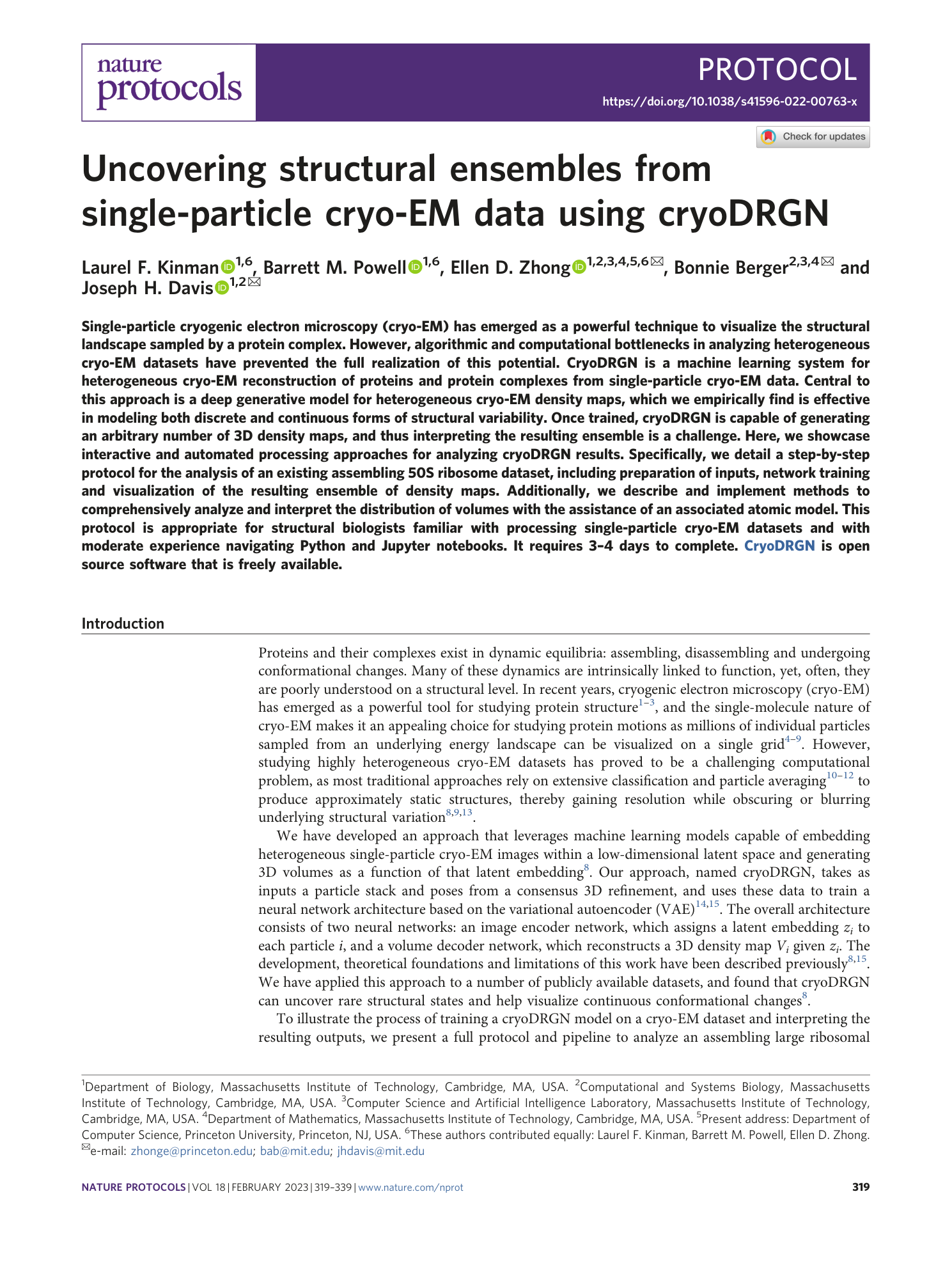
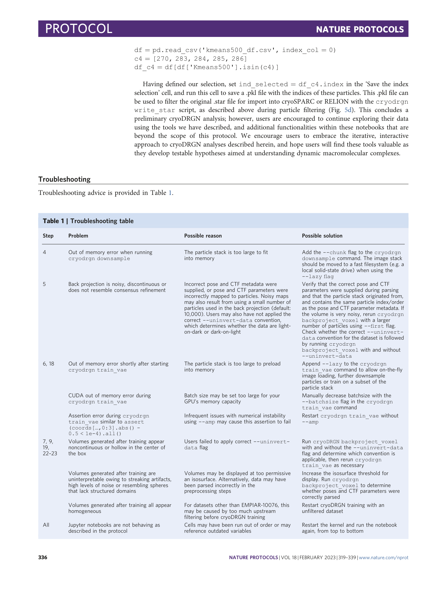
Uncovering structural ensembles from single-particle cryo-EM data using cryoDRGN

Extended Data Fig. 1 Assessing cryoDRGN input parsing.

Comparison of 10,000 cryoDRGN-parsed particles back-projected at D = 128 px (left) with the unsharpened map from cryoSPARC’s homogeneous refinement (right).

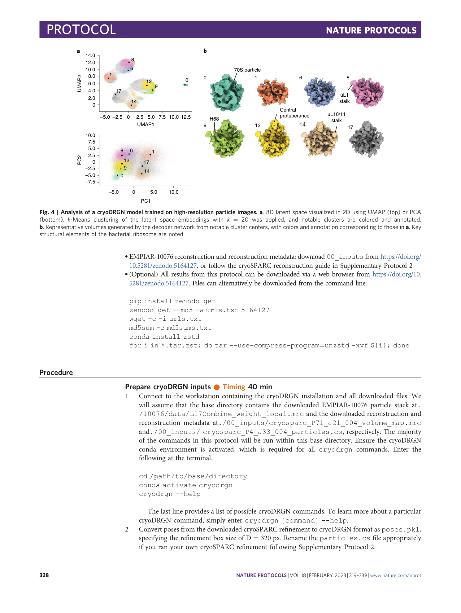
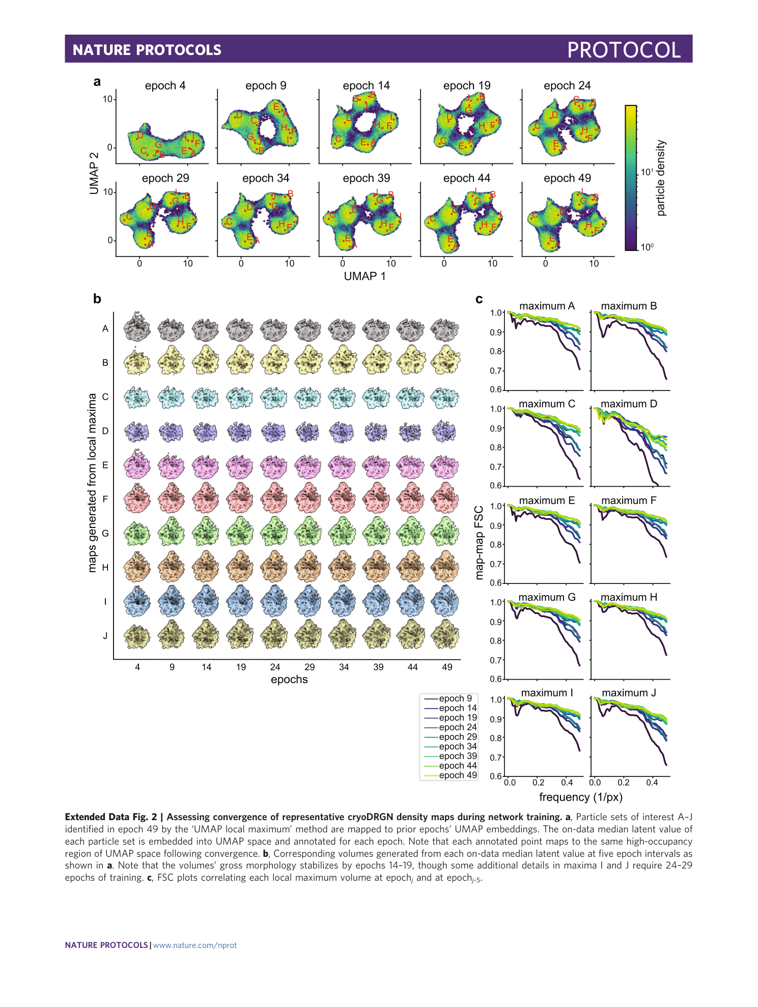
Extended Data Fig. 2 Assessing convergence of representative cryoDRGN density maps during network training.

a , Particle sets of interest A–J identified in epoch 49 by the ‘UMAP local maximum’ method are mapped to prior epochs’ UMAP embeddings. The on-data median latent value of each particle set is embedded into UMAP space and annotated for each epoch. Note that each annotated point maps to the same high-occupancy region of UMAP space following convergence. b , Corresponding volumes generated from each on-data median latent value at five epoch intervals as shown in a . Note that the volumes’ gross morphology stabilizes by epochs 14–19, though some additional details in maxima I and J require 24–29 epochs of training. c , FSC plots correlating each local maximum volume at epoch j and at epoch j -5 .

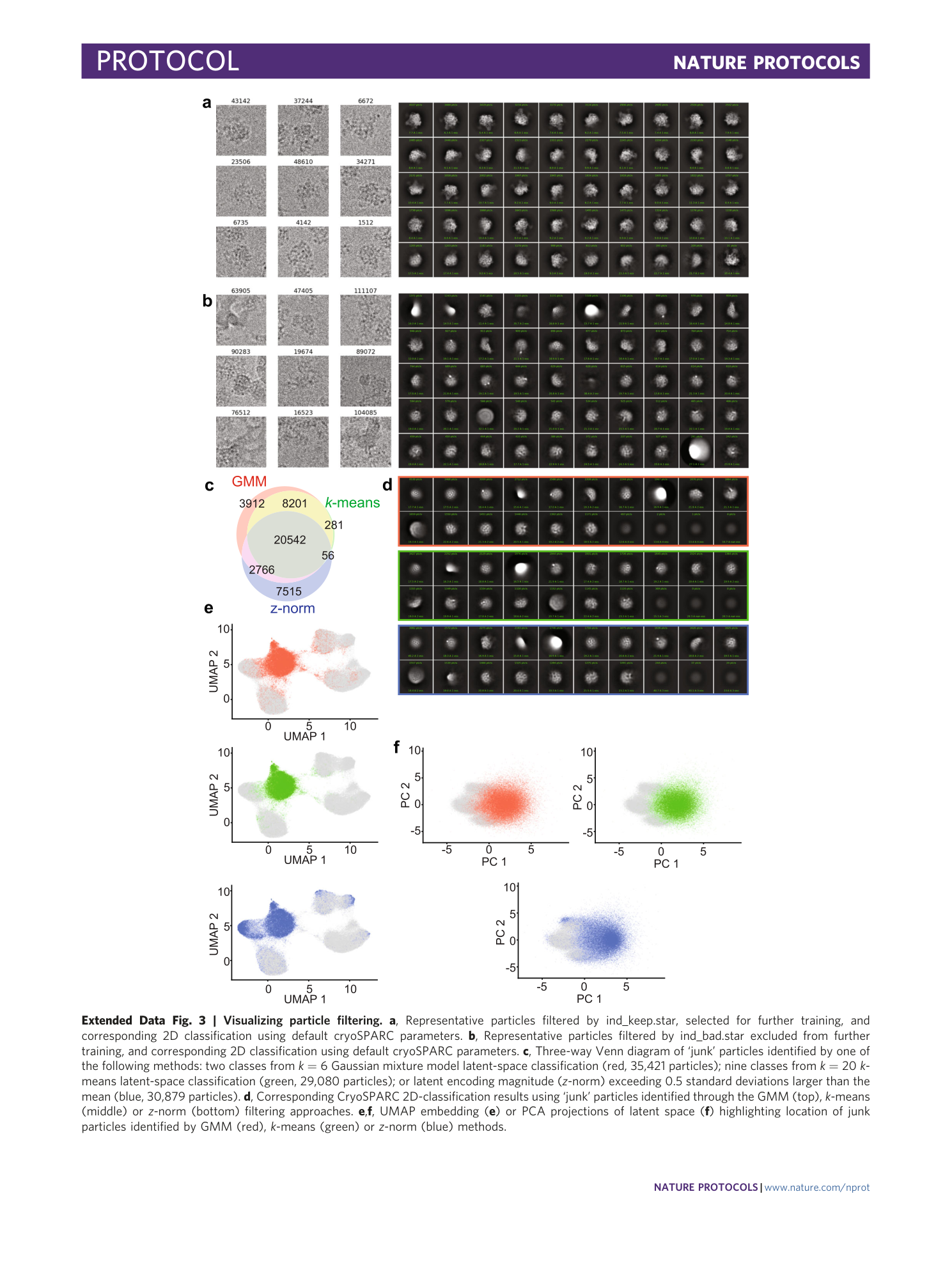
Extended Data Fig. 3 Visualizing particle filtering.

a , Representative particles filtered by ind_keep.star, selected for further training, and corresponding 2D classification using default cryoSPARC parameters. b , Representative particles filtered by ind_bad.star excluded from further training, and corresponding 2D classification using default cryoSPARC parameters. c , Three-way Venn diagram of ‘junk’ particles identified by one of the following methods: two classes from k = 6 Gaussian mixture model latent-space classification (red, 35,421 particles); nine classes from k = 20 k -means latent-space classification (green, 29,080 particles); or latent encoding magnitude ( z -norm) exceeding 0.5 standard deviations larger than the mean (blue, 30,879 particles). d , Corresponding CryoSPARC 2D-classification results using ‘junk’ particles identified through the GMM (top), k -means (middle) or z -norm (bottom) filtering approaches. e , f , UMAP embedding ( e ) or PCA projections of latent space ( f ) highlighting location of junk particles identified by GMM (red), k -means (green) or z -norm (blue) methods.

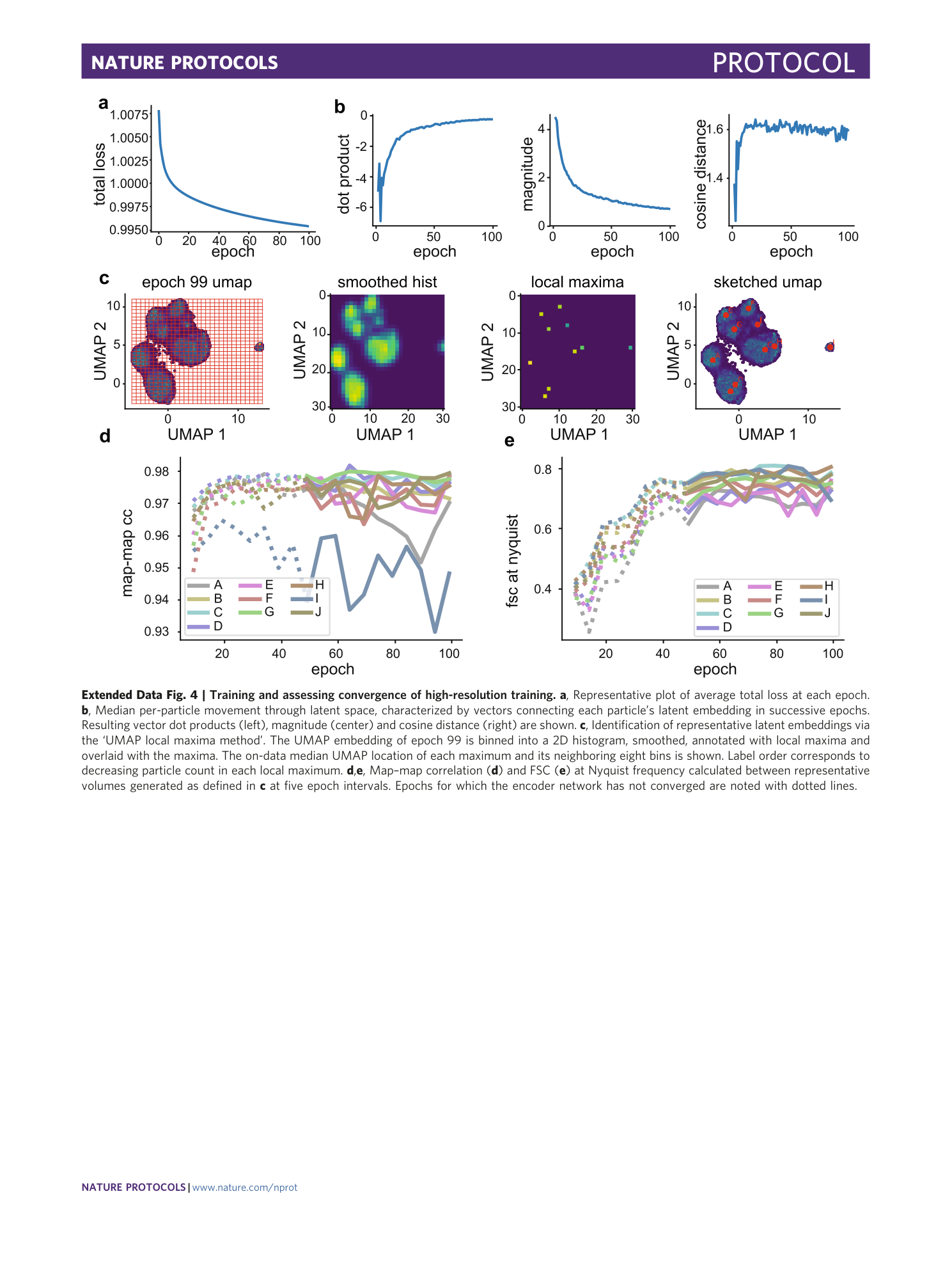
Extended Data Fig. 4 Training and assessing convergence of high-resolution training.

a , Representative plot of average total loss at each epoch. b , Median per-particle movement through latent space, characterized by vectors connecting each particle’s latent embedding in successive epochs. Resulting vector dot products (left), magnitude (center) and cosine distance (right) are shown. c , Identification of representative latent embeddings via the ‘UMAP local maxima method’. The UMAP embedding of epoch 99 is binned into a 2D histogram, smoothed, annotated with local maxima and overlaid with the maxima. The on-data median UMAP location of each maximum and its neighboring eight bins is shown. Label order corresponds to decreasing particle count in each local maximum. d , e , Map–map correlation ( d ) and FSC ( e ) at Nyquist frequency calculated between representative volumes generated as defined in c at five epoch intervals. Epochs for which the encoder network has not converged are noted with dotted lines.

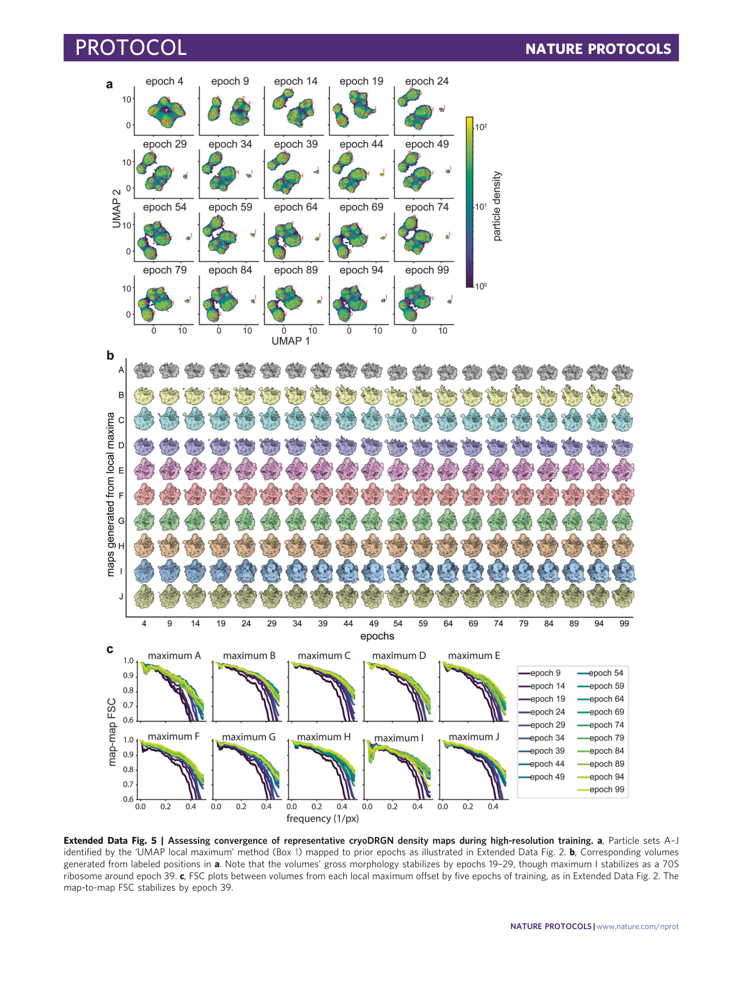
Extended Data Fig. 5 Assessing convergence of representative cryoDRGN density maps during high-resolution training.

a , Particle sets A–J identified by the ‘UMAP local maximum’ method (Box 1 ) mapped to prior epochs as illustrated in Extended Data Fig. 2 . b , Corresponding volumes generated from labeled positions in a . Note that the volumes’ gross morphology stabilizes by epochs 19–29, though maximum I stabilizes as a 70S ribosome around epoch 39. c , FSC plots between volumes from each local maximum offset by five epochs of training, as in Extended Data Fig. 2 . The map-to-map FSC stabilizes by epoch 39.

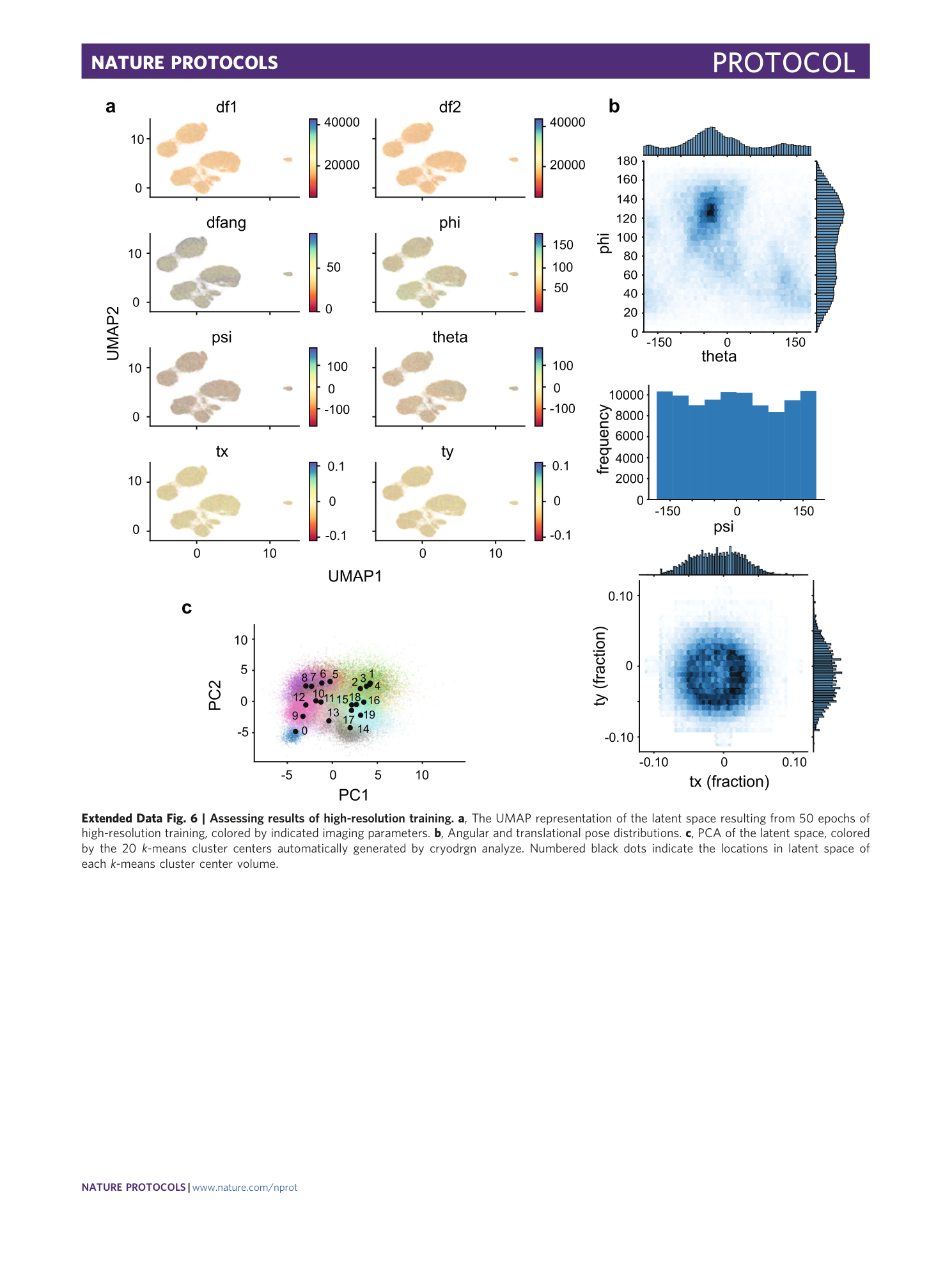
Extended Data Fig. 6 Assessing results of high-resolution training.

a , The UMAP representation of the latent space resulting from 50 epochs of high-resolution training, colored by indicated imaging parameters. b , Angular and translational pose distributions. c , PCA of the latent space, colored by the 20 k -means cluster centers automatically generated by cryodrgn analyze. Numbered black dots indicate the locations in latent space of each k -means cluster center volume.

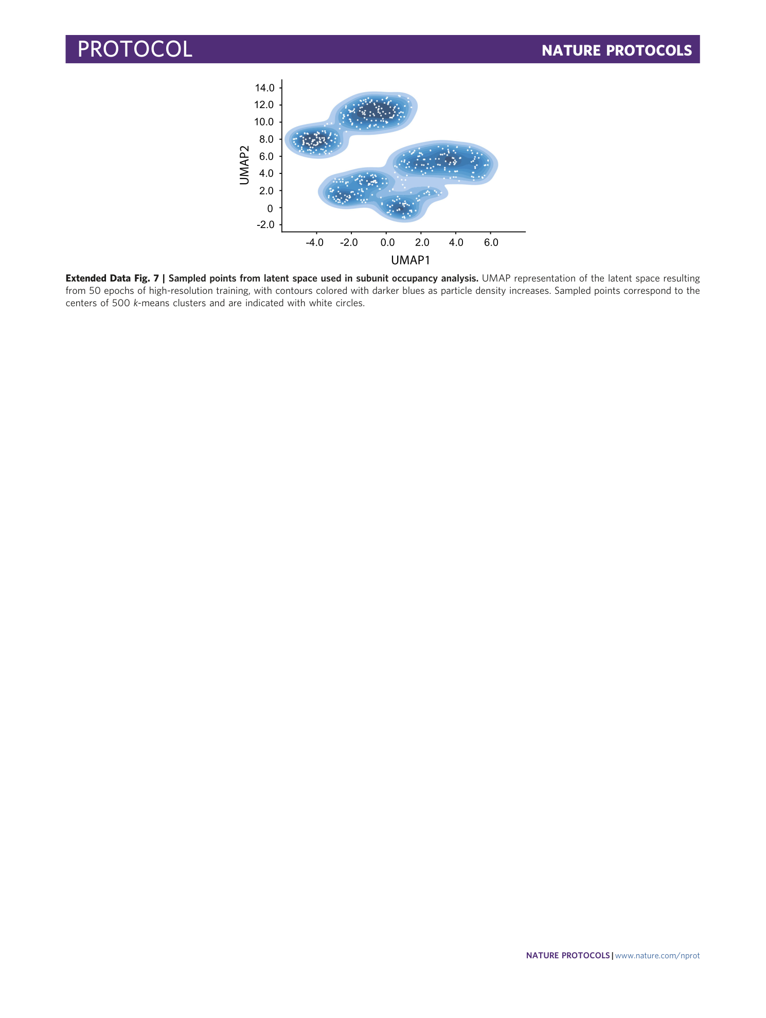
Extended Data Fig. 7 Sampled points from latent space used in subunit occupancy analysis.

UMAP representation of the latent space resulting from 50 epochs of high-resolution training, with contours colored with darker blues as particle density increases. Sampled points correspond to the centers of 500 k -means clusters and are indicated with white circles.

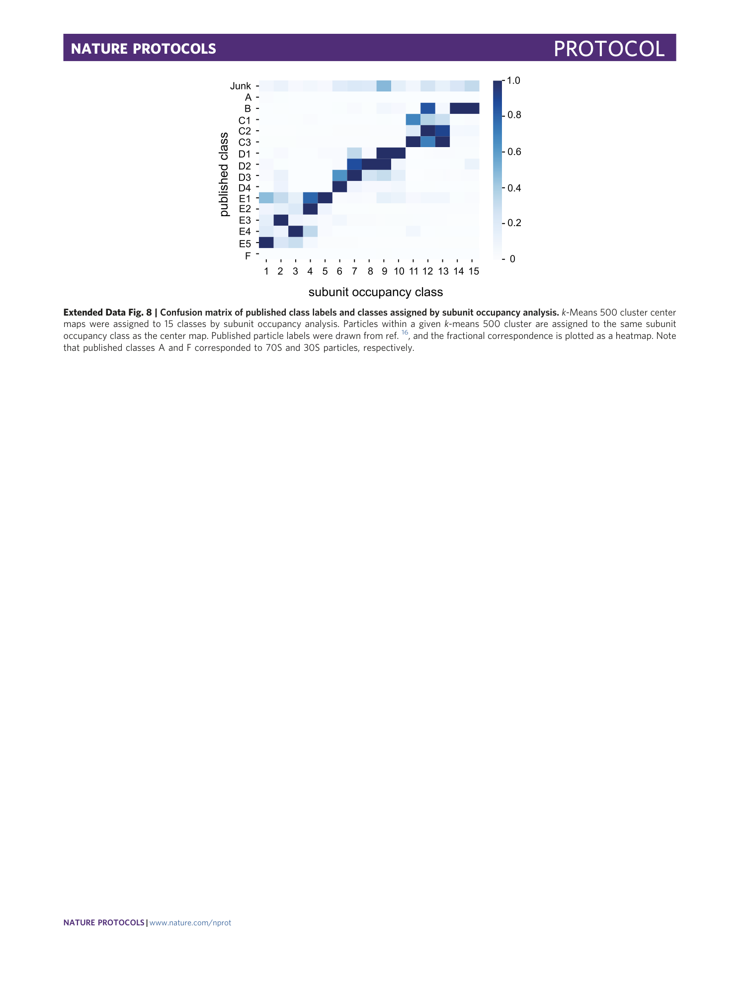
Extended Data Fig. 8 Confusion matrix of published class labels and classes assigned by subunit occupancy analysis.

k -Means 500 cluster center maps were assigned to 15 classes by subunit occupancy analysis. Particles within a given k -means 500 cluster are assigned to the same subunit occupancy class as the center map. Published particle labels were drawn from ref. 16 , and the fractional correspondence is plotted as a heatmap. Note that published classes A and F corresponded to 70S and 30S particles, respectively.

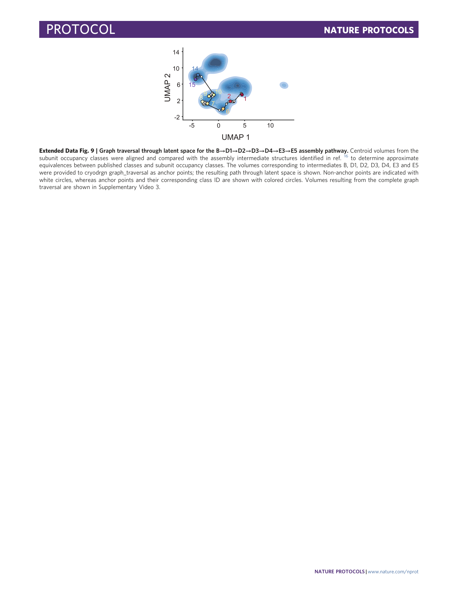
Extended Data Fig. 9 Graph traversal through latent space for the B→D1→D2→D3→D4→E3→E5 assembly pathway.

Centroid volumes from the subunit occupancy classes were aligned and compared with the assembly intermediate structures identified in ref. 16 to determine approximate equivalences between published classes and subunit occupancy classes. The volumes corresponding to intermediates B, D1, D2, D3, D4, E3 and E5 were provided to cryodrgn graph_traversal as anchor points; the resulting path through latent space is shown. Non-anchor points are indicated with white circles, whereas anchor points and their corresponding class ID are shown with colored circles. Volumes resulting from the complete graph traversal are shown in Supplementary Video 3 .

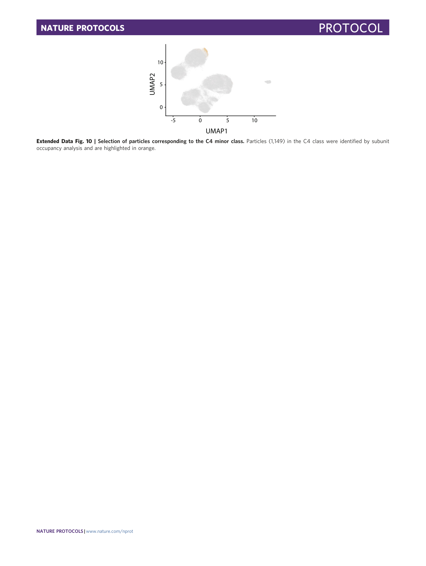
Extended Data Fig. 10 Selection of particles corresponding to the C4 minor class.

Particles (1,149) in the C4 class were identified by subunit occupancy analysis and are highlighted in orange.

Supplementary Information

Supplementary Protocols 1–6 and Supplementary Tables 1 and 2.

Supplementary Video 1

PC1 trajectory from high resolution training . Density maps sampled along PC1 were automatically generated by the cryodrgn analyze command. Volumes are displayed at the same isosurface level, and generated from the 5 th to 95 th PC1 value along the PC1 axis.

Supplementary Video 2

PC2 trajectory from high-resolution training . Density maps sampled along PC2 were automatically generated by the cryodrgn analyze command. Volumes are displayed at the same isosurface level, and generated from the 5 th to 95 th PC2 value along the PC2 axis.

Supplementary Video 3

Graph traversal showing the B→D1→D2→D3→D4→E3→E5 assembly pathway . Graph traversal pathway was generated using the cryodrgn graph_traversal command as described in the protocol. The path taken by the traversal through latent space is shown in Extended Data Figure 9. All volumes are displayed at the same isosurface level.