In-Silico Validation of Biomarkers using ROC and AUC Curve Analysis in R: A Comprehensive Protocol

Biomarkers play a crucial role in the early detection, diagnosis, and management of various diseases. However, the development and validation of reliable biomarkers is a complex and challenging process that requires rigorous evaluation of their analytical and clinical performance. Biomarker validation involves assessing the accuracy, precision, sensitivity, specificity, and reproducibility of the biomarker in a laboratory setting (analytical validation), as well as evaluating its ability to accurately detect or predict the clinical condition of interest in a target population (clinical validation)[1]. In-silico validation, which refers to the computational evaluation of biomarkers using mathematical models, simulations, and data analysis techniques, has become an increasingly important aspect of the biomarker validation process. In-silico validation offers several advantages, including cost-effectiveness, rapid screening of potential biomarkers, hypothesis generation, optimization of assays, and risk assessment. By leveraging computational power and advanced statistical methods, in-silico validation can help identify novel biomarkers, guide the design of subsequent experimental studies, and optimize the performance of biomarker assays. One of the most widely used methods for evaluating the performance of binary classification models, such as those used to predict the presence or absence of a disease based on biomarker levels, is Receiver Operating Characteristic (ROC) curve analysis.[2] ROC curves plot the true positive rate (sensitivity) against the false positive rate (1 - specificity) for different decision thresholds, while the Area Under the ROC Curve (AUC) serves as a summary statistic that represents the overall accuracy of the classification model . ROC and AUC curve analysis provide valuable insights into the performance of biomarkers and help in the selection of optimal cutoff values for clinical decision-making.[3]The objective of this protocol is to provide a comprehensive guide for the in-silico validation of biomarkers using ROC and AUC curve analysis in R, a widely used programming language for statistical computing and graphics. The protocol will cover the necessary steps for data preprocessing, exploratory data analysis, ROC and AUC curve generation, and performance evaluation of biomarkers. By following this protocol, researchers and clinicians can effectively assess the potential of biomarkers for their intended applications and make informed decisions about their clinical utility.

The input file for the in-silico validation protocol should be in CSV (Comma-Separated Values) format, obtained from differential gene expression (DGE) analysis. The file must compulsorily contain two columns: "gene_id" and "logFC". The "gene_id" column should contain the unique identifiers for each gene, while the "logFC" column should provide the log fold change values for each gene, indicating the relative expression between two conditions (e.g., disease vs. control).

install.packages("readr") ): This command installs the readr package, which provides functions to read

rectangular data like CSV files efficiently.

install.packages("pROC") ): This command installs the pROC package, which is used for computing and visualizing Receiver Operating Characteristic (ROC) curves and the Area Under the Curve (AUC).

install.packages("dplyr") ): This command installs the dplyr package, which offers a set of tools for data manipulation and transformation.

> library(readr)
> library(pROC)
> library(dplyr)

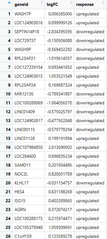
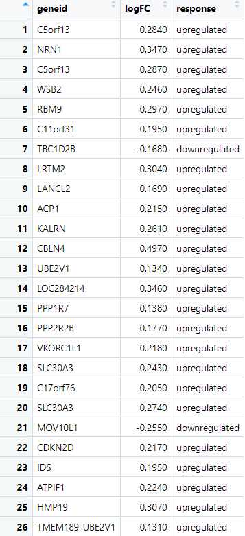
Start with two datasets, one being the test data set and one being a universal dataset. Each must contain only geneid and logFC columns. The first picture depicts Test dataset and second picture shows the universal dataset respectively.

Importing dataset :

read.csv("dge_ALZ.csv") : Reads the dge_ALZ.csv file into a data frame called dge_ALZ which refers to the test dataset.

read.csv("udata1_ALZ.csv") ): Reads the udata1_ALZ.csv file into a data frame called udata1_ALZ which is the universal dataset.

> dge_ALZ <- read.csv("dge_ALZ.csv")
> udata1_ALZ <- read.csv("udata1_ALZ.csv")

Convert Gene IDs to Character Type: After reading the datasets, it is important to ensure that the gene id columns are treated as character type. This is because gene ID values, which represent gene identifiers, are often alphanumeric and need to be recognized as such to facilitate accurate data merging and manipulation. By converting the gene ID columns in both dge_ALZ and udata1_ALZ data frames to character type, we prevent any potential issues that might arise from treating these identifiers as numerical values. This step is critical for maintaining the integrity of the data and ensuring that subsequent merging operations work correctly.

> dge_ALZ$geneid <- as.character(dge_ALZ$geneid)
> udata1_ALZ$geneid <-as.character(udata1_ALZ$geneid)

Create a Response Variable Based on logFC : Next, we create a new column that categorizes each gene based on its logFC value, labeling them as either "upregulated" or "downregulated." This categorization transforms the continuous logFC values into a binary format, which is necessary for defining the response variable required for ROC analysis. By creating this response variable, we set the stage for evaluating the classification performance between the two datasets.

  >   dge_ALZ$response <- ifelse(dge_ALZ$logFC> 0, "upregulated", "downregulated")
  >   udata1_ALZ$response <-ifelse(udata1_ALZ$logFC > 0, "upregulated","downregulated")

Creation of response variable based log FC : The first picture depicts Test dataset and second picture shows the universal dataset respectively.

Merge the Data Frames on geneid : The next step involves merging the two datasets based on the geneid column. By performing an inner join on geneid, we combine the datasets into a single data frame, ensuring that each row corresponds to a unique gene present in both datasets. We also add suffixes to the column names to distinguish between the logFC values from dge_ALZ and udata1_ALZ. This merged dataset allows us to directly compare the logFC values and response variables across the two sources, providing the necessary structure for subsequent ROC curve analysis.

> merged1 <- merge(dge_ALZ, udata1_ALZ, by = "geneid", suffixes = c("_dge", "_udata1"))

Check the Structure of the Merged Data Frame : The str(merged1) function in R is used to display the internal structure of the merged1 data frame. This command is particularly useful for understanding the composition and attributes of the data frame after merging two datasets.

> str(merged1)

Print the Frequency Table of response_dge : This step is performed to get a better understanding of the number of downregulated and upregulated genes respectively.

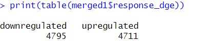
print(table(merged1$response_dge))

Rename logFC Columns: Renaming columns in a data frame is an important step in data preparation to ensure clarity and consistency, especially when dealing with merged datasets with overlapping column names. Here, the columns logFC_dge and logFC_udata1 in the merged1 data frame are renamed to Logfc_dge and Logfc_udata1, respectively. This involves identifying the indices of the columns to be renamed using the which function, and then assigning new, standardized names. This step enhances readability and avoids confusion in later analysis stages, ensuring the data frame is easy to understand and work with, thus facilitating accurate data manipulation and interpretation.

> colnames(merged1)[which(colnames(merged1)== "logFC_dge")] <- "Logfc_dge"
> colnames(merged1)[which(colnames(merged1)== "logFC_udata1")] <- "Logfc_udata1"

Check for Required Columns : This conditional statement checks if the columns Logfc_dge and Logfc_udata1 exist in the merged1 data frame. If either column is missing, the stop() function terminates the execution with an error message. This step ensures data integrity before proceeding with the analysis.

> if(!("Logfc_dge" %in%colnames(merged1)) | !("Logfc_udata1" %in% colnames(merged1))) {
+    stop("Logfc columns not found in merged1")
+ }

The roc() function from the pROC package creates a ROCcurve object roc1 using the response_dge as the true class labels and Logfc_udata1 as the predictor values. The levels parameter specifies the order of the response categories, and direction indicates the direction of comparison. The auc() function calculates the Area Under the Curve (AUC) for the ROC curve, which is printed using cat().

  >  roc1 <- roc(merged1$response_dge,merged1$Logfc_udata1, levels = c("downregulated",
"upregulated"), direction = "<")
 >  cat("AUC for DGE vs UDATA1: ", auc(roc1), "\n")

Finally, the plot() function visualizes the ROC curve, with customization for color and line width. The blue

line represents DGE vs udata.

>    plot(roc1, col = "blue", main ="ROC Curves", lwd = 2)

To perform the Mann-Whitney test in GraphPad Prism, organize your data into two columns for each group and input it into the data table. Click "Analyze," select "Nonparametric tests," and choose the "Man nWhitney test." Ensure the option to compare medians is selected, then click "OK" to run the analysis. Review the output for the U statistic and p-value; a p-value < 0.05 indicates a significant difference. Finally, report the U statistic, p-value, and median differences.[4,5]

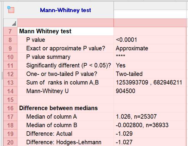
 The results of the Mann-Whitney test indicate a highly significant difference in biomarker levels between the test samples and the universal dataset. The median biomarker level in the test samples (Column A) is significantly higher than that in the universal dataset (Column B), with a difference of approximately 1.029 units. This finding suggests that the biomarker may be a useful indicator for distinguishing between the two groups, potentially supporting its role in diagnostic or prognostic applications related to the condition being studied. These results provide strong evidence for the validity of the biomarker in the context of your research, indicating that it may be effective in differentiating between the populations represented by the two groups.