Determination of G-protein–coupled receptor oligomerization by molecular brightness analyses in single cells
Ali Işbilir, Robert Serfling, Jan Möller, Romy Thomas, Chiara De Faveri, Ulrike Zabel, Marco Scarselli, Annette G. Beck-Sickinger, Andreas Bock, Irene Coin, Martin J. Lohse, Paolo Annibale
G-protein-coupled receptors
oligomerization
fluorescence imaging
molecular brightness
single-cell analysis


Extended
Extended Data Fig. 1 Use of fluorescent ligands to label receptor of interest.
Confocal image of the basolateral membrane of a HEK293-AD cell expressing the Y 2 -receptor C-terminally labeled with EYFP (left) and labeled with 1 μM TAMRA-Ahx(5-24)NPY (center) followed by washout. Right, Upon displacement with 10 μM unlabeled Ahx(5-24)NPY, the fluorescent ligand is almost entirely displaced within tens of seconds. Scale bar, 10 μm.
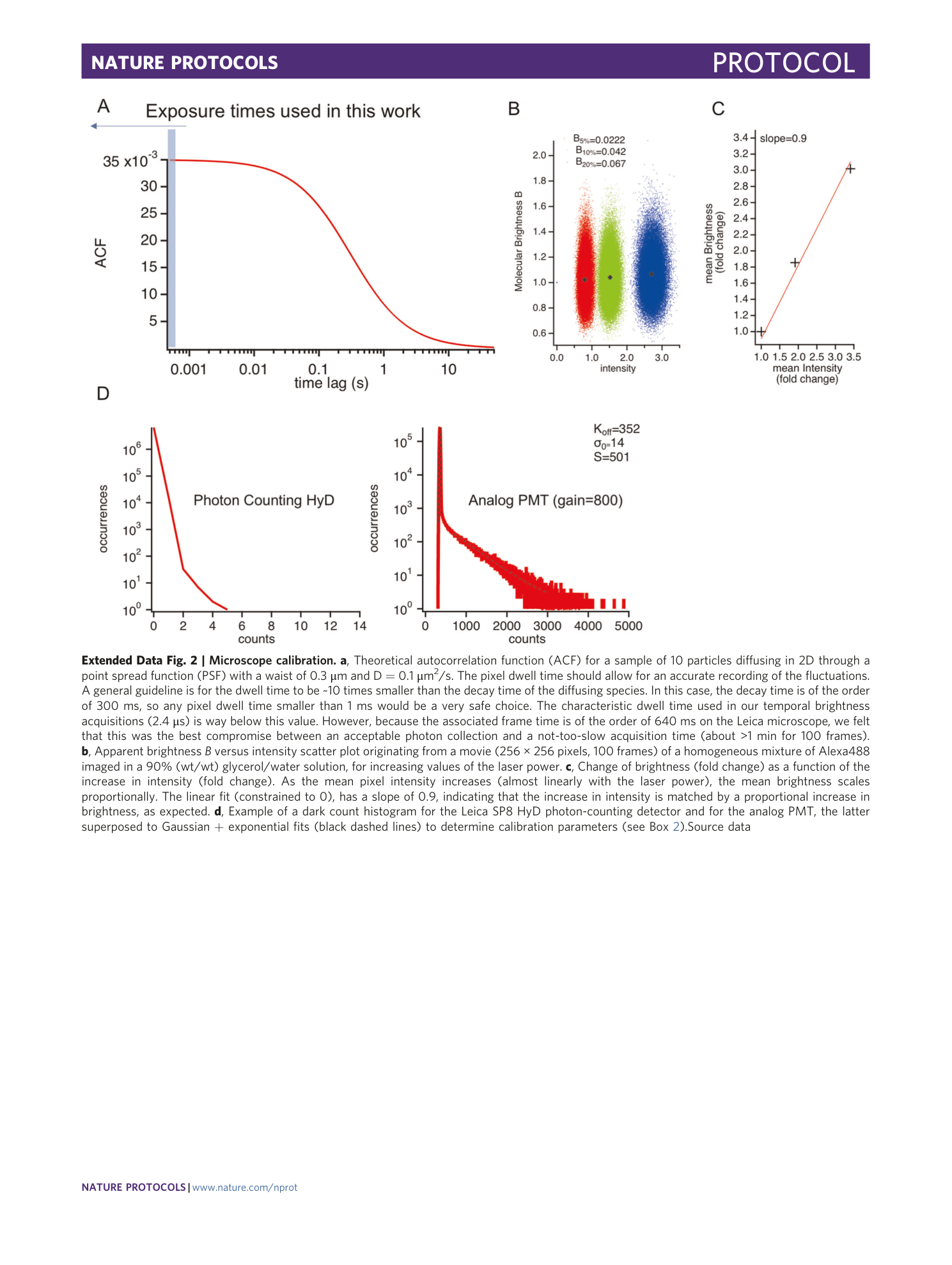
Extended Data Fig. 2 Microscope calibration.
a , Theoretical autocorrelation function (ACF) for a sample of 10 particles diffusing in 2D through a point spread function (PSF) with a waist of 0.3 μm and D = 0.1 μm 2 /s. The pixel dwell time should allow for an accurate recording of the fluctuations. A general guideline is for the dwell time to be ~10 times smaller than the decay time of the diffusing species. In this case, the decay time is of the order of 300 ms, so any pixel dwell time smaller than 1 ms would be a very safe choice. The characteristic dwell time used in our temporal brightness acquisitions (2.4 μs) is way below this value. However, because the associated frame time is of the order of 640 ms on the Leica microscope, we felt that this was the best compromise between an acceptable photon collection and a not-too-slow acquisition time (about >1 min for 100 frames). b , Apparent brightness B versus intensity scatter plot originating from a movie (256 × 256 pixels, 100 frames) of a homogeneous mixture of Alexa488 imaged in a 90% (wt/wt) glycerol/water solution, for increasing values of the laser power. c , Change of brightness (fold change) as a function of the increase in intensity (fold change). As the mean pixel intensity increases (almost linearly with the laser power), the mean brightness scales proportionally. The linear fit (constrained to 0), has a slope of 0.9, indicating that the increase in intensity is matched by a proportional increase in brightness, as expected. d , Example of a dark count histogram for the Leica SP8 HyD photon-counting detector and for the analog PMT, the latter superposed to Gaussian + exponential fits (black dashed lines) to determine calibration parameters (see Box 2 ).
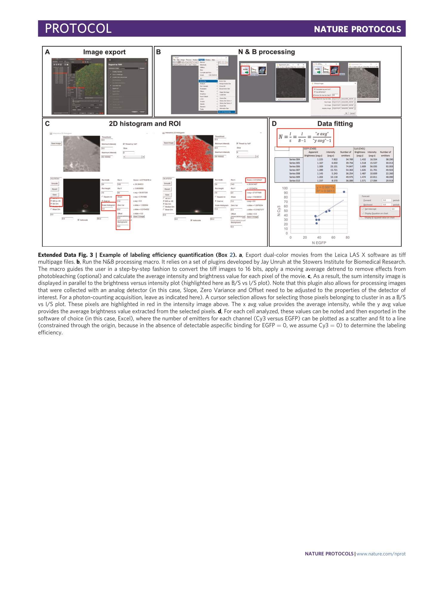
[ Extended Data Fig. 3 Example of labeling efficiency quantification (Box 2 ). ](https://www.nature.com/articles/s41596-020-00458-1/figures/11)
a , Export dual-color movies from the Leica LAS X software as tiff multipage files. b , Run the N&B processing macro. It relies on a set of plugins developed by Jay Unruh at the Stowers Institute for Biomedical Research. The macro guides the user in a step-by-step fashion to convert the tiff images to 16 bits, apply a moving average detrend to remove effects from photobleaching (optional) and calculate the average intensity and brightness value for each pixel of the movie. c , As a result, the sum intensity image is displayed in parallel to the brightness versus intensity plot (highlighted here as B/S vs I/S plot). Note that this plugin also allows for processing images that were collected with an analog detector (in this case, Slope, Zero Variance and Offset need to be adjusted to the properties of the detector of interest. For a photon-counting acquisition, leave as indicated here). A cursor selection allows for selecting those pixels belonging to cluster in as a B/S vs I/S plot. These pixels are highlighted in red in the intensity image above. The x avg value provides the average intensity, while the y avg value provides the average brightness value extracted from the selected pixels. d , For each cell analyzed, these values can be noted and then exported in the software of choice (in this case, Excel), where the number of emitters for each channel (Cy3 versus EGFP) can be plotted as a scatter and fit to a line (constrained through the origin, because in the absence of detectable aspecific binding for EGFP = 0, we assume Cy3 = 0) to determine the labeling efficiency.
