Bioinformatic Analysis to Investigate Metaproteome Composition Using Trans-Proteomic Pipeline
Steven He, Steven He, Shoba Ranganathan, Shoba Ranganathan
Abstract
With evidence emerging that the microbiome has a role in the onset of many human diseases, including cancer, analyzing these microbial communities and their proteins (i.e., the metaproteome) has become a powerful research tool. The Trans-Proteomic Pipeline (TPP) is a free, comprehensive software suite that facilitates the analysis of mass spectrometry (MS) data. By utilizing available microbial proteomes, TPP can identify microbial proteins and species, with an acceptable peptide false-discovery rate (FDR). An application to a publicly available oral cancer dataset is presented as an example to identify the viral metaproteome on the oral cancer invasive tumor front. © 2022 The Authors. Current Protocols published by Wiley Periodicals LLC.
Basic Protocol 1 : Collection of data and resources
Basic Protocol 2 : Analysis of MS data using TPP
Basic Protocol 3 : Analysis of TPP output using R in RStudio
INTRODUCTION
Since the advent of the Human Microbiome Project in 2007 (Turnbaugh et al., 2007), there has been growing research interest in the human microbiome, which refers to the collective aggregate of all microorganisms, including the fungal mycobiome, colonizing on/within human tissues such as the skin, digestive tract, and genitalia. The loss of biodiversity and disruption of microbial homeostasis within these microbial communities, otherwise known as dysbiosis, has since been associated with a wide range of diseases and health conditions, including inflammatory bowel disease (Ni, Wu, Albenberg, & Tomov, 2017), autism spectrum disorders (Kang et al., 2017), pre-term birth (Proctor et al., 2019), and a wide range of cancers (Aykut et al., 2019; Picardo, Coburn, & Hansen, 2019). By studying the metaproteome, which refers to the collective proteome encoded by the microbiome, researchers are able to gain new insights into the microbial compositions associated with different disease states, and also identify differentially expressed functional pathways, if any.
The current paper aims to assist interested researchers in performing metaproteomic analyses using publicly available datasets from repositories, such as ProteomeXchange (Vizcaíno et al., 2014), where MS data is available for a wide range of human diseases, often having only been analyzed in the context of the human proteome. Additional use of the programming language R (Ihaka & Gentleman, 1996) and the Trans-Proteomic Pipeline (TPP), which is a free, high-quality suite of processing tools for the analysis of mass spectrometry (MS) data (Deutsch et al., 2011, 2015), is also explained in this paper. TPP is freely available from the Seattle Proteome Center website (http://tools.proteomecenter.org/wiki/index.php?title=Software:TPP).
Basic Protocol 1: COLLECTION OF DATA AND RESOURCES
Here we describe how to access and download various data resources required for analysis, including the collection of MS data, reference data, and taxonomic information, from the most common publicly available databases.
The Proteomics IDEntifications (PRIDE) database is one of the most common MS data repositories, and while other specialized databases also exist based on their disease classification, such as the Clinical Proteomic Tumor Analysis Consortium (CPTAC) data portal (https://proteomics.cancer.gov/data-portal), which holds data from various cancer tumors (Edwards et al., 2015), these will not be discussed here. Of note, annotation quality varies by dataset, as does the methodology implemented in data acquisition, which should be taken into consideration when planning your own analyses. In particular, it is recommended to select datasets where mechanical disruption (e.g., ultrasonication, bead beating) and detergent (e.g., SDS) have been used for protein extraction (Zhang & Figeys, 2019).
The UniProt (https://www.uniprot.org/proteomes/) database is one of the largest repositories for protein reference sequences (Bateman, 2019). UniProt has the advantage of providing a comprehensive, high-quality, and freely accessible resource of protein sequence and functional information. It also incorporates both the manually annotated and curated SwissProt resource as well as the computationally analyzed TrEMBL data, awaiting full manual annotation. UniProt is also regularly updated and contains microbial (bacterial, viral as well as fungal) proteomes. While the use of existing reference data has the advantage of being easily generalized to most experimental designs, it comes at the expense of database specificity. Other methods to prepare reference databases include the use of prior sample metagenome/metatranscriptome data for construction, or of alternative reference database sources that are specific to certain biological niches. Several examples of such human and murine microbiome databases, which can substitute for UniProt, have been provided in Table 1.The databases selected for inclusion here all have protein FASTA sequence files readily available for reference database construction. While the level of protein annotation for the mouse reference gut microbiome (MRGM; Kim et al., 2021) is somewhat lacking, it still remains one of the more comprehensive murine gut reference sources. While bacterial reference data is readily available from these databases, there currently remain limited options for fungal and viral components of the microbiome in these repositories, representing potential avenues for future research and development. Additionally, it is important to note that as new organisms continue to be sequenced, reference databases need to be updated regularly. To construct up-to-date and niche reference databases, alternative methods of database construction, comprehensively reviewed elsewhere (Blakeley-Ruiz & Kleiner, 2022), may need to be adopted.
| Database | Utility | Limitations |
| Expanded human oral microbiome database (Escapa et al., 2018) |
|
- Lack of information regarding fungal and viral species |
| Unified human gastrointestinal protein catalog (Almeida et al., 2021) |
|
- Lack of information regarding fungal and viral species - Not readily able to map species information to existing NCBI taxonomy IDs |
|
Mouse oral microbiome database (Joseph et al., 2021) |
|
- Lack of information regarding fungal and viral species - Evidence of updates, though schedule/frequency is unclear |
|
Mouse reference gut microbiome (Kim et al., 2021) |
|
- Lack of information regarding fungal and viral species - Lack of protein annotation in .faa FASTA files - Not readily able to map species information to existing NCBI taxonomy IDs - Evidence of updates, though schedule/frequency is unclear |
Finally, the National Center for Biotechnology Information (NCBI) taxonomy database (https://www.ncbi.nlm.nih.gov/taxonomy/) is one of the largest sources of taxonomic information (Schoch et al., 2020), and also is used by UniProt for taxonomy.
The current protocol topic will be broken down into the following:
- 1.Collection of raw MS data from PRIDE
- 2.Collection of microbial proteomes from UniProt for reference database creation
- 3.Collection of taxonomic information from NCBI.
Necessary Resources
Hardware
- Any computer system with Internet access and a browser. Depending on the size of the datasets to be downloaded, additional storage may be required in the form of external hard drives.
Software
- For File Transfer Protocol (FTP) downloads, depending on the organization of the data, the freely available software Filezilla may be used to streamline the download of many files. Filezilla is freely available at https://filezilla-project.org/ and is supported on Windows, Mac OS, and Linux. Additionally, software capable of extracting files from .gz file formats is required. 7-zip is a free option available at https://www.7-zip.org/. Depending on the size of the microbial database being implemented, additional software capable of reading and editing large text files, such as EmEditor (https://www.emeditor.com), is also recommended.
Collection of raw MS data from PRIDE
1.Using your Internet browser, navigate to the PRIDE database (https://www.ebi.ac.uk/pride/) (Martens et al., 2005). Enter a search query to call relevant datasets. If a publication has uploaded its dataset to PRIDE, this can instead be called by entering its PRIDE identifier. This is often in the format “PXD”, followed by a 6-digit identifier (e.g., PXD123456).
2.Clicking on an entry will bring up an information summary about the dataset. Scrolling down to the bottom of the page will show the project files that are available for download. The project files from PXD007232 (https://www.ebi.ac.uk/pride/archive/projects/PXD007232), an MS study on oral cancer (Carnielli et al., 2018), are shown as an example in Figure 1.
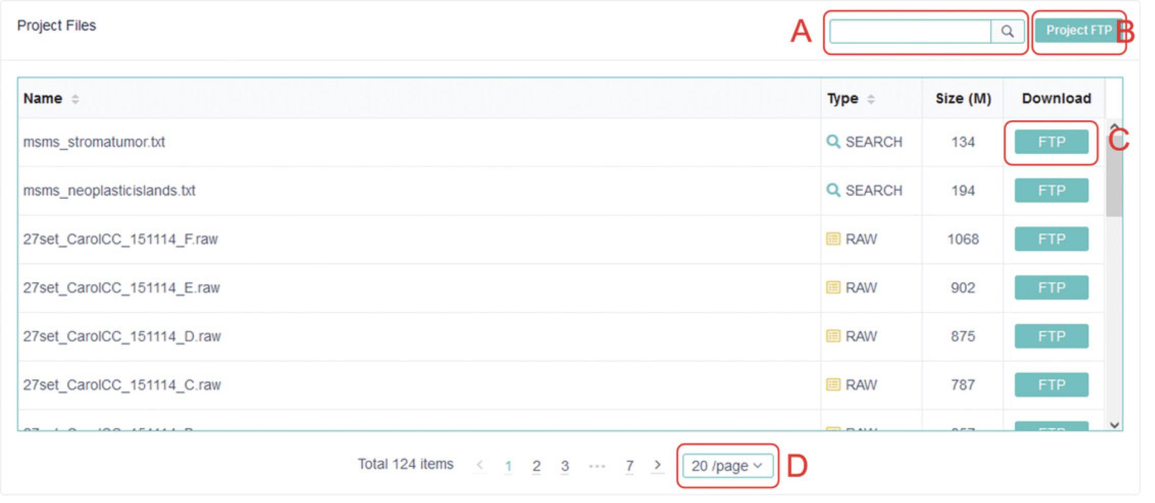
3.Individual files from a project dataset can be selectively downloaded by clicking “FTP” next to the particular file. When there are a large number of files to download, it is recommended to click “Project FTP” and utilize Filezilla FTP download software, freely available from https://filezilla-project.org/.
4.Clicking “Project FTP” will open a new window with a list of all available files for a particular project. Open Filezilla and copy the website URL into the “Host” field in Filezilla to establish a remote connection with the PRIDE FTP server (Fig. 2A).
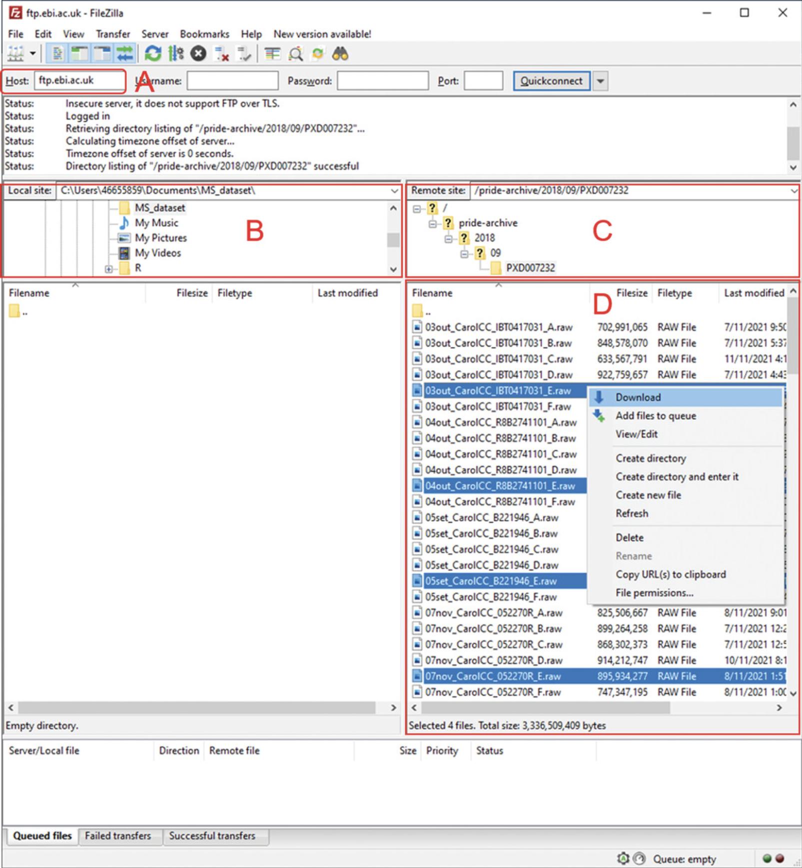
5.Once the connection is established, use the local navigation pane to select the destination to which files will be downloaded (Fig. 2B). If the URL has correctly been entered from step 4, there should be no need to use the remote site navigation (Fig. 2C), and the project files should be visible (Fig. 2D). After selecting all desired files, right-click and select “Download” to begin downloading the selected files. This can be more convenient when a large number of MS data files are required to be downloaded.
Collection of microbial proteomes from UniProt for reference database creation
6.Open your preferred Internet browser and navigate to UniProt proteomes (https://www.uniprot.org/proteomes).
7.On the left-hand sidebar under “Filter by”, select “Reference proteomes” (Fig. 3A).
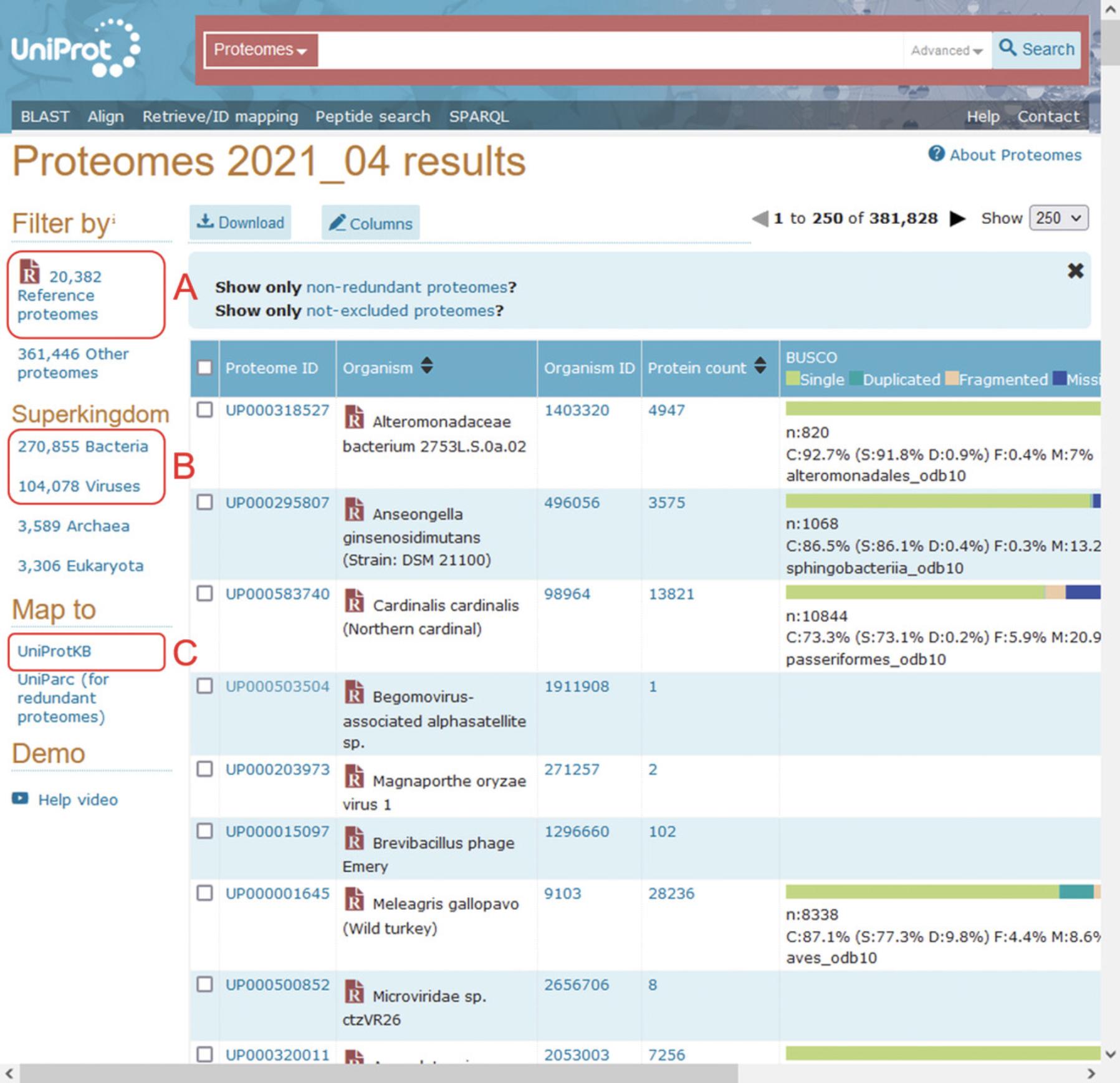
8.On the same left-hand sidebar, select “Bacteria” or “Viruses” to filter by the desired microbe. Here, “Viruses” will be used as an example (Fig. 3B).
9.With all viral reference proteomes now selected, on the left-hand sidebar under “Map to”, select “UniProtKB”. This will show all protein entries mapping to the selected viral proteomes. Selecting “Download” from above the results window will allow all returned entries to be downloaded into a single FASTA file, which can be used as the reference database. For the example reference database, all viral reference proteomes were downloaded in FASTA format, totaling 594,570 protein sequences (515,513 viral proteins, 79,057 human proteins; files downloaded 15th Feb 2022).
10.Of note, as fungi are grouped in Eukaryota on the sidebar, a separate query, “taxonomy:Fungi [4751]”, must be entered into the search bar to obtain fungal sequences. After this, select “Reference proteomes” and map to “UniProtKB” as previously described before downloading as FASTA.
11.Assuming that metaproteomic analysis is being performed on human samples, in order to improve FDR, a copy of the human reference proteome should also be downloaded (available from https://www.uniprot.org/proteomes/UP000005640) and appended to the previously downloaded FASTA file reference database using a copy and paste command. If an alternate host species is being used (e.g., mouse), then the corresponding reference proteome should be appended instead.
Collection of taxonomic information from NCBI
12.The National Center for Biotechnology Information (NCBI) taxonomy database, on which UniProt's taxonomy is based, can be downloaded from https://ftp.ncbi.nih.gov/pub/taxonomy/new_taxdump/. Download one of either “new_taxdump.tar.Z”, “new_taxdump.tar.gz”, or “new_taxdump.zip”; all three contain the same data but are intended to provide convenience in unpacking on different operating environments. Opening the “taxdump_readme.txt” will provide more information.
13.Extract “rankedlineage.dmp” from the downloaded file. The .dmp file contains the taxonomic information for all organisms in the NCBI database, and will be used in Basic Protocol 3
Basic Protocol 2: ANALYSIS OF MS DATA USING TPP
Here we describe the use of various TPP modules for the analysis of the downloaded MS data using the constructed reference database. This includes the conversion of the MS data, database searching, and then peptide and protein validation. A breakdown of the following workflows will be provided in this protocol:
- 1.Starting up TPP
- 2.Conversion of proprietary file formats using msconvert
- 3.Database searching using Comet
- 4.Peptide validation using PeptideProphet
- 5.Protein inference using ProteinProphet.
Necessary Resources
Hardware
- A computer system with minimum 16 GB RAM and i7 or newer processor is recommended for the analysis, to reduce processing time. Depending on the size of the dataset to be analyzed, additional memory storage may also be required.
Software
- TPP software is used for the MS data analysis. It can be freely downloaded from the Seattle Proteome Center website (http://tools.proteomecenter.org/wiki/index.php?title=Software:TPP) and is supported on Windows, Mac OS, and Linux. The current protocol will assume TPP (version 6.0.0) is being run using the Windows OS.
Starting up TPP
1.Prior to running the TPP software, the requisite files need to be moved into the correct TPP directories. Navigate to the TPP folder (default installation path is to the C: drive).
2.Move the downloaded RAW MS files into the TPP/data folder and the FASTA format reference database to TPP/data/dbase.
3.From the Desktop, open TPP by double clicking the “Trans-Proteomic Pipeline” shortcut icon (created by default during installation). TPP will open in a new Internet browser window. Alternatively, open your preferred internet browser and enter the URL http://localhost:10401/tpp/; this assumes default settings during the TPP installation.
4.Select “Petunia”, which is the main TPP graphical user interface (GUI). When prompted to login, enter “guest”, which acts as both the default user name and password.
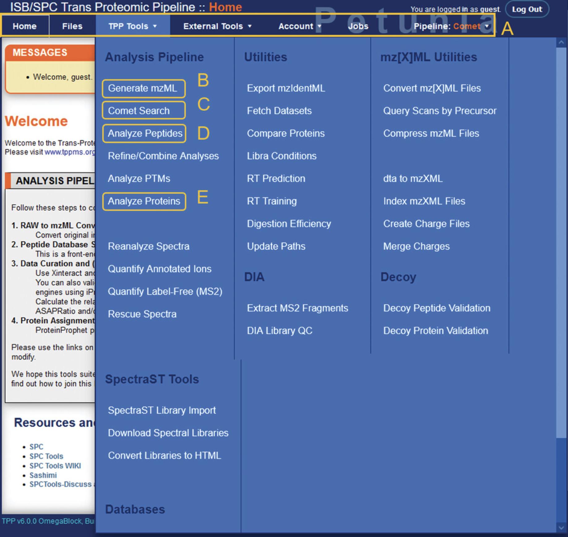
5.From the main TPP home page, links to the primary tools for MS analysis can be found under “TPP Tools” on the menu bar (Fig. 4).
Conversion of proprietary file formats using msconvert
6.First, the RAW MS data files need to be converted to mzML format. Select the “Generate mzML” option under TPP Tools to open the msconvert module.
7.Select the input file format (default is Thermo RAW) and then select “Add Files” to open a new navigation screen. Navigate to your TPP data directory and select the RAW MS files to be converted. Doing so will return you to the previous screen.
8.Click “convert to mzML” to begin the job. This process may take several minutes to several hours depending on the number of files to convert and specifications of your computer.
Output files
9.Once the msconvert module has finished running, .mzML files corresponding to each data file input will be produced. The output files will appear in the same directory as the input files.
Database searching using Comet
10.From the TPP home page, select “Comet Search” under TPP Tools to open the Comet database search module. In the Comet screen, there will be three prompts to choose mzML input files, a Comet parameters file, and a sequence database (Fig. 5).
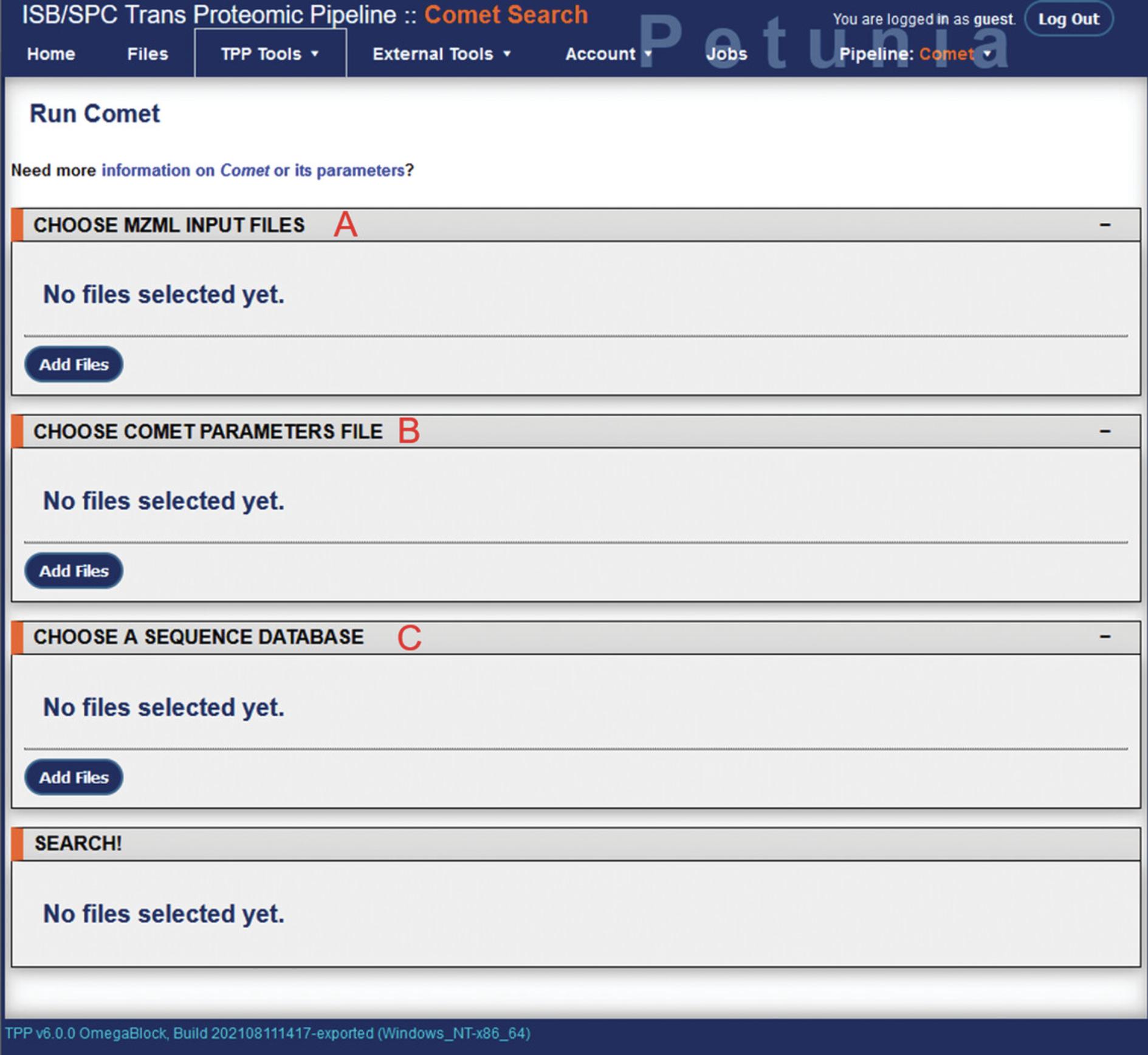
11.Under “choose mzML input files”, click “Add Files” to open up a new directory navigation screen. Navigate to the .mzMLfiles produced by msconvert and select them as input files. This will return you to the Comet search page.
12.Select “Add Files” under “choose Comet parameter files” to similarly open directory navigation. A default set of Comet parameters can be found in TPP/data/param/comet.params. This can be edited by selecting the “Params” link next to the file. From here, various parameters of the database search can be adjusted such as peptide mass tolerance, decoy search, missed cleavages, and amino acid variable modifications. The Comet search parameters used for the example analysis can be found in Supplementary File 2 (see Supporting Information).
13.Selecting “Add Files” under “Choose a sequence database” will open directory navigation. Navigate to the reference database prepared earlier (TPP/data/dbase) and select it.
14.With the input files, Comet parameters, and reference database selected, the “Run Comet Search” button will appear at the bottom of the page. Clicking this will begin the database search. Checking the “Preview” box next to this will show the command issued to TPP, but will not run the actual analysis. Depending on the number of files to be analyzed, size of the database, search parameters, and computer hardware being used, the database search may take several minutes to several hours. Using the example data here, the Comet database search required approximately 3 hr to complete.
15.While running, the progress of the analysis can be viewed from the Jobs tab on the menu bar (Fig. 4A).
Output files
16.Once the analysis is complete, a pep.xml file will be produced for each .mzML file in the same directory as the Comet parameters file used. The results of each analysis, prior to peptide validation and protein inference, can be viewed using the File option on the TPP menu bar.
Peptide validation using PeptideProphet
17.From the TPP Home page, using the menu bar select “TPP Tools” > “Analyze Peptides” to access the PeptideProphet module (Fig. 6; Ma, Vitek, & Nesvizhskii, 2012). There will be multiple fields corresponding to file input, output options, and PeptideProphet settings, followed by options for additional software modules including iProphet, PTMProphet, XPRESS, ASAPRatio, and Libra. While these modules have useful applications depending on the analysis (iProphet for concatenation of multiple database searching, PTMProphet for post-translational modifications, XPRESS and ASAPRatio for relative quantitation of isotopically labeled data, and Libra for isobaric-tagged quantitation), they will not be explored here.
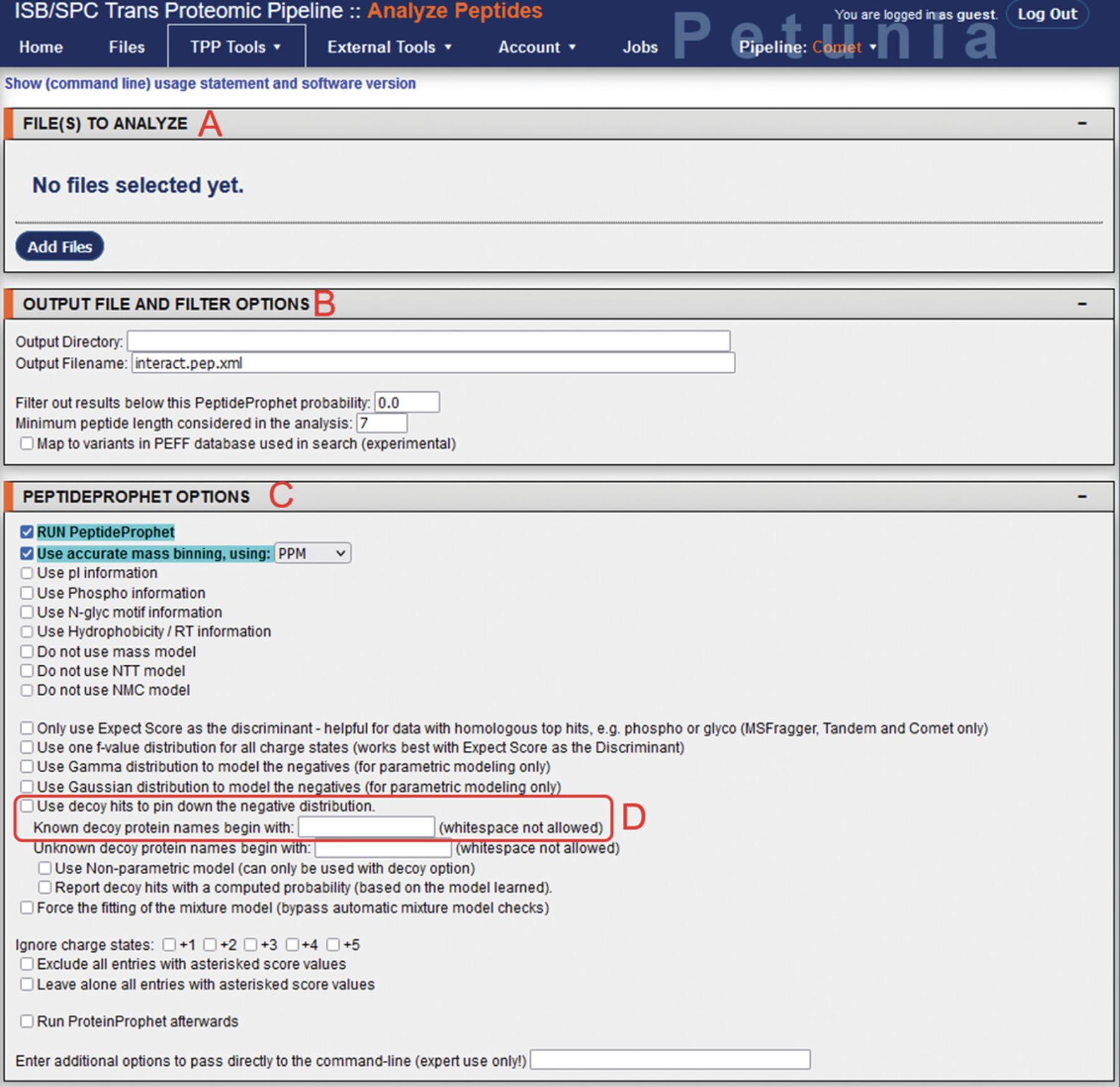
18.In the “Files to analyze” section, selecting “Add Files” will open up the directory navigator. Locate and select the pep.xml file outputs from the Comet search for input into PeptideProphet.
19.Under “Output file and filter options”, select the directory where the output files will be produced, and the output filename (when changing the output filename, ensure that it ends with the .pep.xml extension).
20.Under “PeptideProphet Options”, additional parameters can be modified. The “Run PeptideProphet” and “Use accurate mass binning, using: PPM” settings are enabled by default. If a decoy search was used during the Comet database search, enable the “Use decoy hits to pin down the negative distribution” option and input the decoy prefix used into the “Known decoy protein names begin with” field.
21.Click Run XInteract to initiate the analysis. While generally requiring less processing time than the Comet search, depending on the size and number of files to be analyzed, as well as hardware specifications, this step may take a few minutes to a few hours. Using the example data, this analysis required approximately 40 min to complete.
Output files
22.After completion of the analysis, a new pep.xml file (or files) will be produced in the designated output directory. The results can be viewed from the File option on the TPP menu bar.
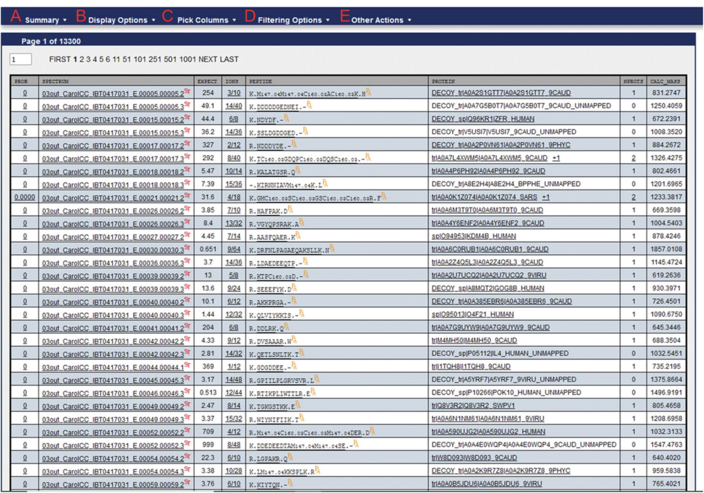
23.Selecting the results will open the PepXML viewer (Fig. 7). Export the results data in .xls format by selecting “Other Actions” > “Export Spreadsheet”. This will produce a new .xls file in the same directory as the pep.XML file.
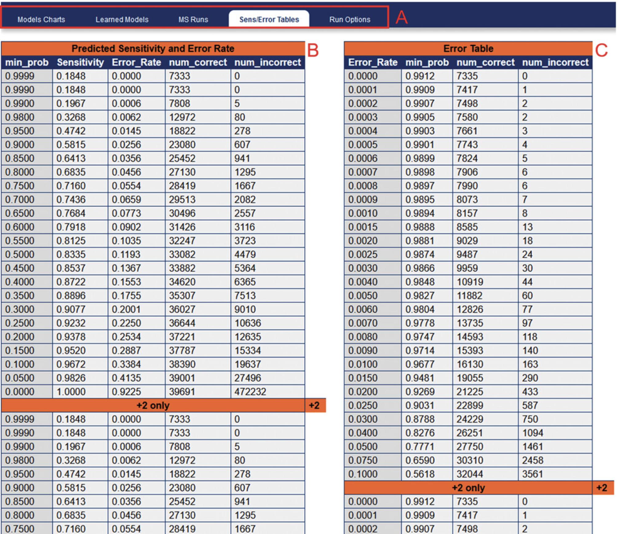
24.In order to determine the FDR for a specified PeptideProphet probability score, navigate to “Other Actions” > “Additional Analysis Info”. This will open a new window containing sensitivity and error rate modeling (Fig. 8). Selecting the Sens/Error Tables tab will show the corresponding predicted FDR (labeled as “Error_Rate”) for a given PeptideProphet probability score.
Protein inference using ProteinProphet
ProteinProphet can also be run immediately after PeptideProphet by selecting “Run ProteinProphet afterwards” under “PeptideProphet” options.
25.From the TPP home page menu bar, select “TPP Tools” > “Analyze Proteins” to access the ProteinProphet module (Fig. 9; Nesvizhskii, Keller, Kolker, & Aebersold, 2003).
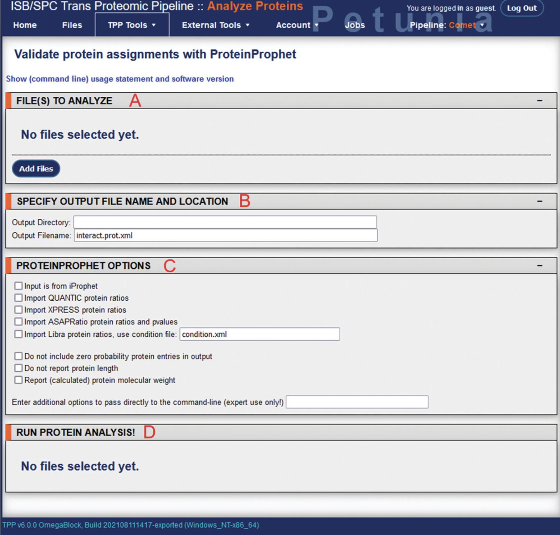
26.Multiple fields will be visible, corresponding to file input, output options, and the ProteinProphet run options.
27.In the “Files to analyze” section, selecting “Add Files” will again open up the directory navigator. Locate and select the pep.xml file outputs from the PeptideProphet analysis for input into ProteinProphet.
28.Under “Specify output file name and location”, the output directory can be changed, as well as the output filename. When changing the output filename, ensure it ends with the .prot.xml extension.
29.Under “ProteinProphet options”, several settings can be adjusted if specific quantitation software applications were used during upstream analysis. By default these parameters are unused.
30.Once input files have been selected, the “Run ProteinProphet” button will appear at the bottom under “Run protein analysis!”. Clicking this will initiate the analysis and bring the user to a new screen showing job progress. While generally requiring less processing time than the Comet search, again depending on the size and number of files to be analyzed, as well as hardware specifications, this step may take a few minutes to a few hours. Using the example data, this analysis step required approximately 2 min to complete.
Output files
31.After completion of the analysis, a new prot.xml file (or files) will be produced in the designated output directory. The results can be viewed from the File option on the TPP menu bar.
32.Selecting the results will open the ProtXML viewer (Fig. 10). The results data can be exported in .tsv format by selecting “File & Info” > “Export TSV”. This will produce a new .tsv file in the same directory as the prot.xml file. The ProteinProphet output of example data using a peptide mass tolerance of 5 ppm can be viewed in Supplementary File 3 (see Supporting Information).
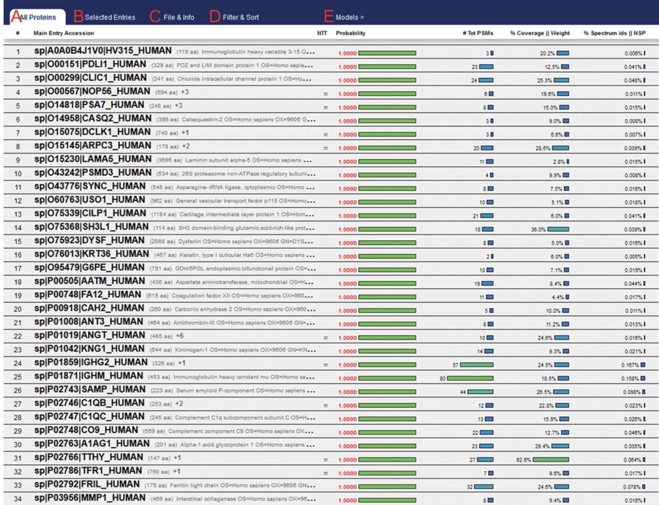
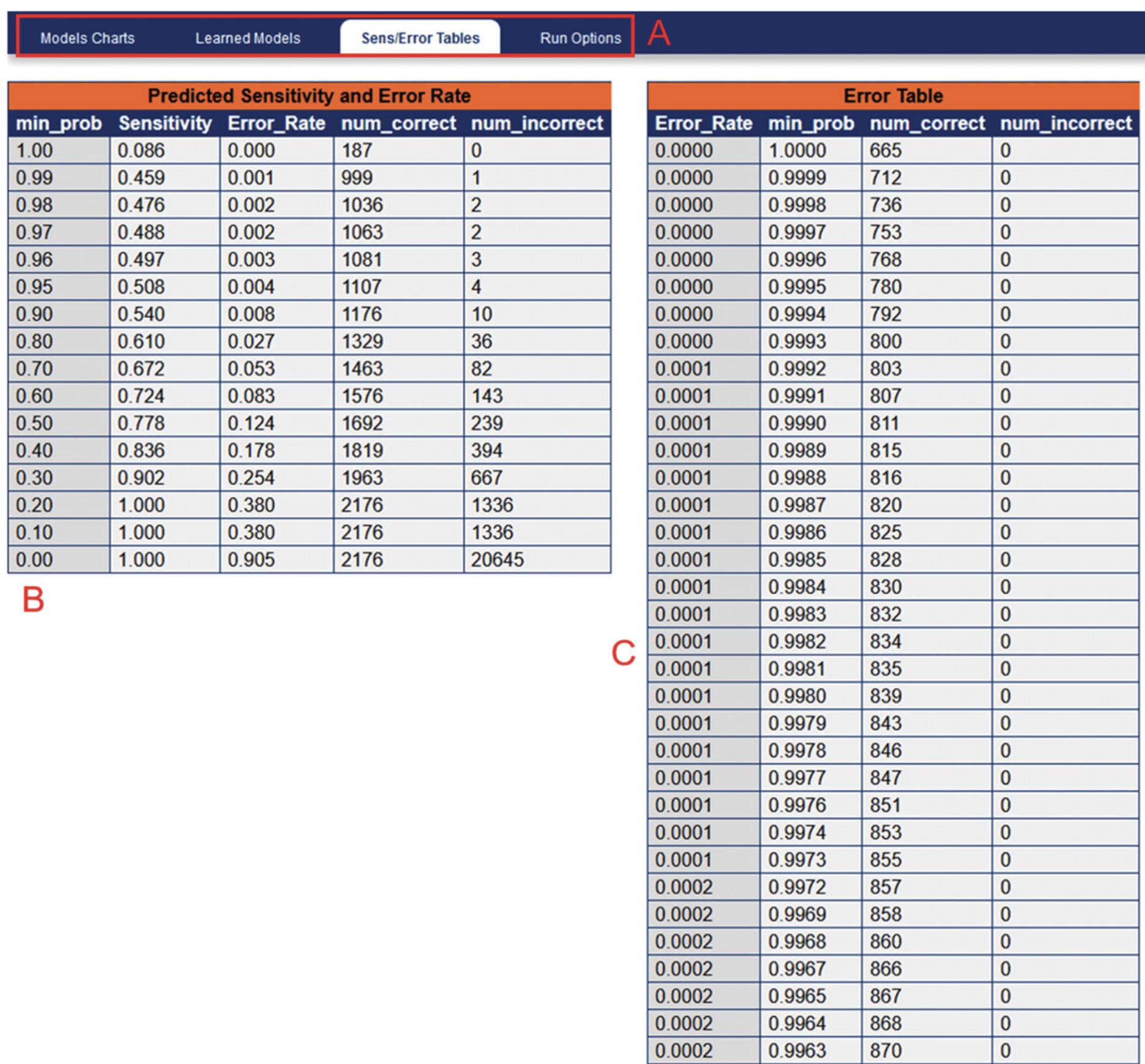
33.In order to determine the FDR for a specified ProteinProphet probability score, click “Models” in the ProtXML viewer menu bar. This will open a new window containing sensitivity and error rate modeling (Fig. 11). Selecting the Sens/Error Tables tab will show the corresponding predicted FDR (labeled as “Error_Rate”) for a given ProteinProphet probability score.
Basic Protocol 3: ANALYSIS OF TPP OUTPUT USING R IN RSTUDIO
R, commonly used with the RStudio Integrated Development Environment (IDE), is a powerful programming language developed primarily for statistical computing and has many applications in the sciences for data analysis and visualization (Ihaka & Gentleman, 1996). This protocol describes the secondary analysis of the TPP ProteinProphet .tsv outputs using RStudio for data processing, and visualization of taxonomic information from inferred microbial species using sunburst plots. The following protocol will be broken up into the following sections:
- 1.Creating a project directory
- 2.Import and filtering of data
- 3.Appending taxonomy information and visualization using sunburst plot.
Necessary Resources
Hardware
See Basic Protocol 1
Software
- Both R and RStudio are software are required, and can be freely downloaded from https://cran.rstudio.com/ and https://www.rstudio.com/products/rstudio/download/, respectively.
- In addition, several R packages are required for this protocol: ‘tidyverse’, ‘plotly’, and ‘data.table’. These can be installed from the console window in RStudio using the “install.packages()” function. Alternatively these can be installed from the menu bar by navigating to “Tools” > “Install Packages…”. R version 4.1.2.and RStudio (ver. 2021.09.01+372) have been used for the current protocol.
Creating a project directory
1.Open RStudio and use the menu bar to navigate to “File” > “New Project”. From here you will have the option of creating a new project from a new or from an existing directory.
2.After creating the new project, move the ProteinProphet .tsv output files (from Basic Protocol 3) into the new project directory. This allows for ease of access, as opening the project automatically defines the working directory as the same as the project directory. An .Rproj-format file should be present in this folder.
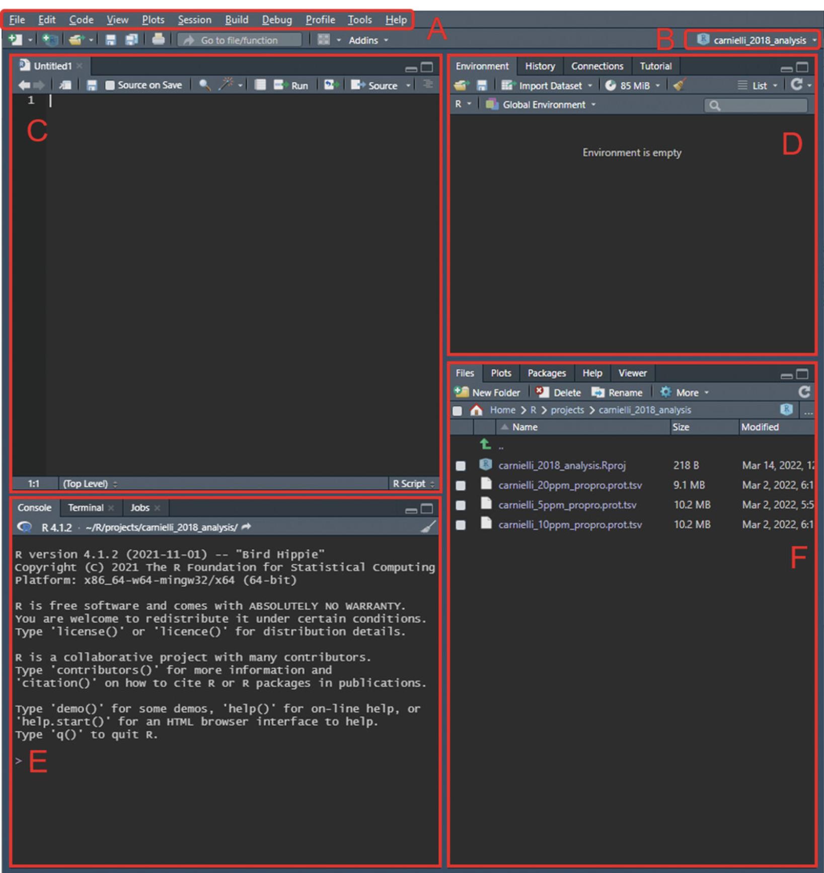
3.With the project open, from the menu bar, navigate to “File” > “New File” > “R Script”, or use the shortcut Ctrl+Shift+N to create a new script for subsequent coding. With a new script open, four panes should be visible (see Fig. 12).
Import and filtering of data
4.Load the packages required in the protocol (tidyverse, data.table, plotly) using the function “library()”.
5.Import the .tsv ProteinProphet outputs and assign them to a variable (e.g., “raw_data”) using the “read_tsv()” function. The imported data can be viewed in the source editor by selecting it from the workspace browse (Fig. 12D) or by using the function “View()”.
6.Once the data has been imported, filtering criteria can be applied in the source editor to remove human entries, protein groups, and low-probability proteins. This can be performed using the filter() function. Example code is shown below, assuming the reference database used was created using UniProt reference data, with ‘#’ denoting comments:
filter_data<-raw_data%>%- #remove HUMAN entries
- filter(!str_detect(protein, "HUMAN")) %>%
- #remove protein groups
- filter(!str_detect(protein, "tr|.tr|.")) %>%
- filter(!str_detect(protein, "sp|.tr|.")) %>%
- filter(!str_detect(protein, "tr|.sp|.")) %>%
- filter(!str_detect(protein, "sp|.sp|.")) %>%
- #remove low prob proteins
- filter(
protein probability>= 0.95)
- filter(
While the ProteinProphet probability threshold shown here is 0.95, this value will differ for each analysis and should be based on the desired FDR threshold in consultation with the ProteinProphet sensitivity and error tables. For the analysis of the example data using a 5 ppm peptide mass tolerance, a probability threshold of 0.96 was used to give FDR = 0.01.
7.New separate columns with species id information can then also be created in this output using the “str_extract()” function. The example code shown below assumes that UniProt sequences were used to construct the reference database, giving the new columns “tax_name” and “tax_id”:
filter_data"protein description", "(?<=OS=).*(?= OX=)") filter_data"protein description","(?<=OX=)[:digit:]*") filter_datatax_id)
8.This analyzed data of high-probability proteins and their associated organism can then be exported using the “write.csv()” function for further interpretation.
Appending of taxonomy information and visualization using sunburst plot
9.Move the “rankedlineage.dmp” file (here, downloaded 4th Feb 2022), extracted in Basic Protocol 1, to the R project directory.
10.Import the .dmp file into R using the “read_tsv()” function. Additional cleaning of the database is performed using the “select()” and “colnames()” functions before mapping the output from step 7 above to the taxonomy database with the “merge()” function:
-
import data and remove unused columns
- db <- read_tsv("rankedlineage.dmp") %>% select(seq(1,by=2,len=10))
-
label database column names with corresponding taxon level
- colnames(db) <- c("tax_id", "tax_name", "species", "genus", "family", "order", "class", "phylum", "kingdom", "superkingdom")
-
map output data to taxonomy database
taxa_data<- merge(db,filter_data, by="tax_id")
The examples here assume that a UniProt reference database was used in Basic Protocol 3.Taxon identifiers (tax_id) remain mostly consistent between Uniprot and NCBI; however, there may be occasional inconsistencies. Make sure to compare the number of rows for consistency following the merge; in this example we compare “filter_data” and “taxa_data” and find that 17 out of 2098 entries (<1% of total data) are not successfully merged. Using the “anti_join()” function can allow for unmerged rows to be identified, after which they can be manually checked based on “tax_name” and other info. Following manual checking, only two rows were unable to be merged.
If an alternate reference database was used for the primary MS analysis (i.e., not from Uniprot), an alternative taxonomy database other than NCBI may be required, and differences in the data structure may require modifications to the example code shown here. For example, the expanded Human Oral Microbiome Database has its own taxon database (https://www.homd.org/download#taxon) that contains additional columns not present in the NCBI taxonomy database.
11.Convert the data frame into a data table using the “as.data.table()” function. Additionally, assign N/A values as “Unclassified” (i.e., no classification present in the taxonomy database being used) and create a “count” column to view how many protein hits map back to a particular organism. Using this “counts” column, a threshold can be implemented to increase confidence in species inference based on desired acceptance criteria (i.e., only keep species identified by two or more proteins).
data_table<- as.data.table(taxa_data)data_table[,count := .N, by = . (tax_name)]data_table<-data_table%>% filter(count >= 2)data_table[is.na(data_table)] <- "Unclassified"taxa_data<- taxa_data[,c("kingdom", "phylum", "class", "order", "family", "genus", "tax_name")]
12.Prior to sunburst plot visualization using the plotly package, the data has to be converted into an amenable format. This can be performed by defining the function “as.sunburst”, shown in the code below. Execute the function on the output from step 12 above, and then use the “plot_ly()” function to visualize the data:
-
#Define function as.sunburst
-
as.sunburst <- function(dataframe, value_column = NULL, add_root = FALSE){
- require(data.table)
- names_dataframe <- names(dataframe)
- if(is.data.table(dataframe)){
- datatable <- copy(dataframe)
- } else {
- datatable <- data.table(dataframe, stringsAsFactors = FALSE)
- }
- if(add_root){
- datatable[, root := "Total"]
- }
- names_datatable <- names(datatable)
- hierarchy_cols <- setdiff(names_datatable, value_column)
- datatable[, (hierarchy_cols) := lapply(.SD, as.factor), .SDcols = hierarchy_cols]
- if(is.null(value_column) && add_root){
- setcolorder(datatable, c("root", names_dataframe))
- } else if(!is.null(value_column) && !add_root) {
- setnames(datatable, value_column, "values", skip_absent=TRUE)
- setcolorder(datatable, c(setdiff(names_dataframe, value_column), "values"))
- } else if(!is.null(value_column) && add_root) {
- setnames(datatable, value_column, "values", skip_absent=TRUE)
- setcolorder(datatable, c("root", setdiff(names_dataframe, value_column), "values"))
- }
- hierarchy_list <- list()
- for(i in seq_along(hierarchy_cols)){
- current_cols <- names_datatable[1:i]
- if(is.null(value_column)){
- current_datatable <- unique(datatable[, ..current_cols][, values := .N, by = current_cols], by = current_cols)
-
} else {
- current_datatable <- datatable[, lapply(.SD, sum, na.rm = TRUE), by=current_cols, .SDcols = "values"]
- }
- setnames(current_datatable, length(current_cols), "labels")
- hierarchy_list[[i]] <- current_datatable
- }
- current_datatable <- datatable[, lapply(.SD, sum, na.rm = TRUE), by=current_cols, .SDcols = "values"]
-
* hierarchy_datatable <\- rbindlist(hierarchy_list, use.names = TRUE, fill = TRUE)- parent_columns <- setdiff(names(hierarchy_datatable), c("labels", "values", value_column))
- hierarchy_datatable[, parents := apply(.SD, 1, function(x){fifelse(all(is.na(x)), yes = NA_character_, no = paste(x[!is.na(x)], sep = ":", collapse = " - "))}), .SDcols = parent_columns]
- hierarchy_datatable[, ids := apply(.SD, 1, function(x){paste(x[!is.na(x)], collapse = " - ")}), .SDcols = c("parents", "labels")]
- hierarchy_datatable[, c(parent_columns) := NULL]
- return(hierarchy_datatable)
-
}
-
#Execute function on data
-
plot_data<- as.sunburst(data_table) -
#Create sunburst plot
-
plot_ly(data=
plot_data, ids=∼ids, labels=∼labels, parents=∼parents, values=∼values, type='sunburst', branchvalues='total', textinfo='label+percent root', maxdepth=5)
Multiple arguments in the function can be modified to change the appearance of the plot, the most common being the “maxdepth” argument to determine the maximum taxon levels shown at a given time, as well as the “textinfo” argument, which display any combination of “label”, “value”, “percent root”, “percent parent”, and “current path,” among others.
Output files
13.Executing the above commands will generate a sunburst plot in the Viewer pane (Fig. 12F) with the taxonomic information of species inferred from the MS data. The sunburst plot is interactive, where specific section selections magnify them and their lower levels (Fig. 13).
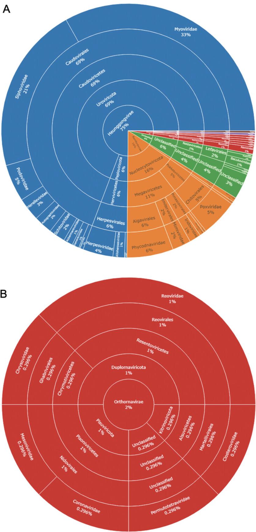
14.A static image of the sunburst plot can be exported by selecting “Export” > “Save as Image” from the Viewer pane toolbar. Alternatively, an image can be created using the bmp(), png(), jpg(), or tiff() functions, depending on the desired image format. The exported image will appear in the project working directory.
15.In addition to creating a static image, an interactive figure can be exported as a .html document by assigning the plot to a variable and using the function “htmlwidgets::saveWidget()”. Example code is shown below:
- sunburst <- plot_ly(data=plot_data, ids=∼ids, labels=∼labels, parents=∼parents, values=∼values, type='sunburst', branchvalues='total', textinfo='label+percent root', maxdepth=5)
- htmlwidgets::saveWidget(as_widget(sunburst),"supp_file4_sunburst.html")
The R script used here for the analysis of the example data can be viewed in Supplementary File 4 (see Supporting Information). Additionally, an interactive version of Figure 13 can also be viewed in Supplementary File 5.
GUIDELINES FOR UNDERSTANDING RESULTS
The protocols in this article aim to assist researchers in analysis of MS data for metaproteomics, and allow for identification of high-probability microbial proteins, as well as insight into the taxonomic composition of the niche being studied. From this basic pipeline, two main outputs are produced: the identified protein list output from ProteinProphet (.tsv format) and an interactable sunburst plot displaying taxonomic information of inferred species (.html format, although static images can also be produced).
The ProteinProphet output contains useful parameters including ProteinProphet probability score, protein length, percentage protein coverage from identified peptides, the number of PSMs used for inference, spectrum ID percentage, and observed peptide sequences. When using a UniProt reference database, additional information will be displayed under protein description corresponding to FASTA entry headers. This includes protein name, reviewed or unreviewed status (sp| and tr|, respectively, denoting Swiss-Prot or TrEMBL sequences), organism (OS), taxonomic identifier (OX), gene name (GN), level of evidence for protein existence (PE), and sequence version information (SV). More information on these parameters can be found at https://www.uniprot.org/help/fasta-headers. It is important to note that this output is an unfiltered list; to obtain a processed list, it is possible to use the command “write.csv()” in R following step 8 of Basic Protocol 3 to export a filtered version of the results. Implementing additional acceptance criteria, such as requiring a minimum of three observed peptides for protein inference, can be used for more conservative analysis. When presenting these results, the version information (where available) and download date of FASTA files used for reference database creation, as well as filtering criteria, should be reported.
The sunburst plot provides a graphical representation of the inferred taxonomic composition for the sample niche being studied. This can be particularly useful for comparison between different conditions (e.g., healthy and disease) to identify differing trends in microbial composition at higher grouped taxa such as the genus or family level, as opposed to the individual species level, which can be challenging to replicate consistently between experiments. Although recommendations exist, there are no concrete guidelines for reporting and interpretation of metaproteomic data (Zhang & Figeys, 2019), and so it is necessary to report the acceptance criteria used for species inference. While the species have been inferred by the presence of two or more unique proteins, the stringency of this can be altered to be more or less conservative, for example by increasing or decreasing the number of proteins required for inference, or by including only reviewed Swiss-Prot proteins instead of both these and hypothetical TrEMBL sequences, with the latter being used here. However, where reference sequences of hypothetical/putative proteins have been used, caution should be taken when drawing conclusions from this data, especially where no other supporting evidence is available. It is important to note that the protocols shown here only identify the presence or absence of a particular inferred species, and that no interpretations or conclusions can be readily made regarding the abundance of an organism between conditions.
As mentioned earlier, there can be significant challenges associated with the interpretation of metaproteomics data. Validity of the results is heavily reliant on the use of appropriate reference databases, as the problem of protein inference, a long-standing issue even in conventional proteomics (Huang, Wang, Yu, & He, 2012), is greatly exacerbated by the presence of many different species in metaproteomics. Indeed, increasing sample complexity has been demonstrated to reduce the number of protein identifications as well as the protein coverage of individual species, and, by extension, the resolution of species inference becomes more challenging as the number of homologous proteins from closely related species increases (Lohmann et al., 2020). The current method overcomes this by using a conservative approach where only unique proteins, based on the reference database, are retained. This comes at a cost, however, with the additional filtering generally resulting in fewer protein identifications. If increased identifications are desired by the user at the cost of resolution, reference databases can be constructed using clustered data from non-redundant databases such as UniRef (Suzek, Huang, McGarvey, Mazumder, & Wu, 2007), or user-defined sequences can be clustered based on similarity to produce custom reference databases using software such as CD-HIT (Li & Godzik, 2006). Further comprehensive review of the challenges and considerations for metaproteomics analyses can be found elsewhere (Heyer et al., 2017; Zhang & Figeys, 2019).
As with any bioinformatic in silico pipeline, additional validation of the results is recommended, whether that be through confirmation using orthogonal techniques—such as metagenomics or culture-based experiments where possible—or by performing your own MS experiments to replicate the observations made using publicly available data.
COMMENTARY
Background Information
Microbiome research has increased dramatically in recent years and has led to many scientific discoveries across a myriad of various diseases, such as a causative role for Campylobacter jejuni in colorectal cancer tumorigenesis (He et al., 2019), and has provided insight into new possible methods for diagnosis and treatment (Cullen et al., 2020).
Here we present a pipeline for metaproteomic analysis using both TPP and R. While this article details the analysis of pre-existing, publicly available MS data, the methodology can also easily be adapted to analyze primary data. While only a basic application of the pipeline is presented here using data-dependent acquisition (DDA) MS data, the advantage of the particular software applications being used is their extremely high capacity for customization; TPP is a robust MS analysis platform that can be additionally used to analyze metaproteomic data where labeling has been applied or data-independent acquisition (DIA) has been used, while R code can similarly be customized specifically to suit the needs of the researcher (Tippmann, 2015). While having these customizations options can be invaluable, it does, however, sacrifice useability when compared to other metaproteomic analysis software such as MetaProteomeAnalyzer (Muth et al., 2015).
We recently used this approach to mine the metaproteomic profile of human plasma in both SARS-CoV-2 (also known as COVID-19) patients and healthy controls from publicly available DDA MS datasets. Here, we observed a loss of bacterial diversity and corresponding increase of viral protein identifications with increasing severity of SARS-CoV-2 infection, ranging from healthy to mild, and then fatal (Alnakli, Jabeen, Chakraborty, Mohamedali, & Ranganathan, 2022).
Critical Parameters and Troubleshooting
Some of the critical parameters of the protocols described above include:
Reference database creation
The creation of a reference database that accurately reflects the niche being studied is of great importance to accurately identify hits. This can be a delicate balancing act; while larger databases tend to be more comprehensive, an increasing search space results in higher FDR and exponentially longer search times. Conversely though, too small a database runs the risk of excluding important or novel organisms and their proteins. Where it may not be possible to create a de novo reference library from metagenomics data of the sample being studied, alternative curated databases exist for specific biological niches such as the eHOMD (Escapa et al., 2018), for the human oral microbiome, and the UHGP (Unified Human Gastrointestinal Protein) catalog (Almeida et al., 2021), for the human gastrointestinal tract. Although providing the least specificity, where no alternative is available, reference proteomes from UniProt can be used to construct the reference database.
Peptide mass tolerance in database search
The peptide mass tolerance within the database search refers to the maximal accepted difference between observed experimental mass and a theoretical mass that is considered a match by the search algorithm. Altering the peptide mass tolerance can drastically affect the search results, and is highly dependent on the instrument being used. Multiple searches can be performed to identify an optimal peptide mass tolerance. To highlight this, Comet database searches were performed with the example data at 5, 10, and 20 ppm peptide mass tolerance, yielding 2098, 161, and 162 unique viral proteins identifications, respectively, after ProteinProphet analysis at an FDR of 0.01.
In addition to these considerations, further possible issues that may arise in the protocol, and potential solutions, are discussed in Table 2.
| Problem | Possible cause | Solution |
| File is unable to be located or opened by TPP or its modules | Certain syntax is not tolerated by TPP and its modules, most notably whitespace | Remove and avoid using spaces in folder or file names. Underscores can be substituted instead (“_”) |
| Long run times using Comet database search | Search space may be too large | If possible, lower the amount of variable modifications in the Comet .params file and/or use a database more targeted to the environment of interest. If the reference database is too large, it is also possible to split this into smaller files and do multiple database searches, before concatenating the results at a later step |
| TPP times out during longer jobs | The default server timeout setting is 18,000 s | Navigate to “TPP/conf/httpd-tpp.conf” and open using Notepad or similar software. Locate the parameter “Timeout 18,000” and change the numeric value as desired (e.g., 604,800 corresponds to 7 days before server timeout). |
| Peptide/ProteinProphet files are not opening in the TPP XML viewer | File extensions have not been correctly provided | Ensure that the PeptideProphet and ProteinProphet outputs have their full respective file extensions of “.pep.xml” and “.prot.xml” |
| Errors in R when filtering protein data and/or mapping of taxonomy | Different database other than UniProt used to construct reference database | The example analysis presented here used UniProt to generate the reference database. Resultantly the UniProt naming structure is reflected in the code and may need to be altered to accurately reflect the delimiters and idiosyncrasies of the database being used. As UniProt uses the NCBI taxonomy database, when using alternative databases to Uniprot, try to identify and use the corresponding taxonomy database (if not NCBI). Again, the code may need to be altered to reflect the data structure (e.g., the number of columns may differ from the NCBI database). |
| Error when generating sunburst plot with plotly, or a blank plot is produced | Data is in an unamenable format for conversion using the “as.sunburst” function | Ensure that there are no missing values in the data, and that columns are ordered top-down in terms of classification level. The example data and script used here is available in Supplementary Files 4 and 5 (see Supporting Information) and can be used for comparison of data tables. |
Acknowledgments
The authors would like to acknowledge the support and insight of both the spctools discussion group and StackOverflow community knowledgebase, as well as the bioinformatics group members (Dr. Amara Jabeen, Mr Aziz Alnakli, and Dr. Rajdeep Chakraborty) for their support. Additionally, S.H. acknowledges Macquarie University for award of the RTP-MRES scholarship which assisted in supporting this work.
Open access publishing facilitated by Macquarie University, as part of the Wiley - Macquarie University agreement via the Council of Australian University Librarians.
Author Contributions
Steven He : conceptualization, data curation, formal analysis, investigation, methodology, software, visualization, writing original draft; Shoba Ranganathan : conceptualization, project administration, resources, supervision, writing review and editing.
Conflict of Interest
The authors declare no conflict of interest.
Open Research
Data Availability Statement
Data derived from public domain resources.
Supporting Information
| Filename | Description |
|---|---|
| cpz1506-sup-0001-raw-data-info.xlsx9.8 KB | Supporting Information 1 |
| cpz1506-sup-0002-comet-5ppm.params9.6 KB | Supporting Information 2 |
| cpz1506-sup-0003-SupMat.tsv7.4 MB | Supporting Information 3 |
| cpz1506-sup-0004-Rscript.R5 KB | Supporting Information 4 |
| cpz1506-sup-0005-sunburst.html4.9 MB | Supporting Information 5 |
Please note: The publisher is not responsible for the content or functionality of any supporting information supplied by the authors. Any queries (other than missing content) should be directed to the corresponding author for the article.
Literature Cited
- Almeida, A., Nayfach, S., Boland, M., Strozzi, F., Beracochea, M., Shi, Z. J., … Finn, R. D. (2021). A unified catalog of 204,938 reference genomes from the human gut microbiome. Nature Biotechnology , 39(1), 105–114. doi: 10.1038/s41587-020-0603-3
- Alnakli, A. A. A., Jabeen, A., Chakraborty, R., Mohamedali, A., & Ranganathan, S. (2022). A bioinformatics approach to mine the microbial proteomic profile of COVID-19 mass spectrometry data. Applied Microbiology , 2(1), 150–164. doi: 10.3390/applmicrobiol2010010
- Aykut, B., Pushalkar, S., Chen, R., Li, Q., Abengozar, R., Kim, J. I., … Miller, G. (2019). The fungal mycobiome promotes pancreatic oncogenesis via activation of MBL. Nature , 574(7777), 264–267. doi: 10.1038/s41586-019-1608-2
- Bateman, A. (2019). UniProt: A worldwide hub of protein knowledge. Nucleic Acids Research , 47(D1), D506–D515. doi: 10.1093/nar/gky1049
- Blakeley-Ruiz, J. A., & Kleiner, M. (2022). Considerations for constructing a protein sequence database for metaproteomics. Computational and Structural Biotechnology Journal , 20, 937–952. doi: 10.1016/j.csbj.2022.01.018
- Carnielli, C. M., Macedo, C. C. S., De Rossi, T., Granato, D. C., Rivera, C., Domingues, R. R., … Paes Leme, A. F. (2018). Combining discovery and targeted proteomics reveals a prognostic signature in oral cancer. Nature Communications , 9(1), 3598.doi: 10.1038/s41467-018-05696-2
- Cullen, C. M., Aneja, K. K., Beyhan, S., Cho, C. E., Woloszynek, S., Convertino, M., … Rosen, G. L. (2020). Emerging priorities for microbiome research. Frontiers in Microbiology , 11(February), 136. doi: 10.3389/fmicb.2020.00136
- Deutsch, E. W., Mendoza, L., Shteynberg, D., Farrah, T., Lam, H., Sun, Z., … Aebersold, R. (2011). A guided tour of the TPP. Proteomics , 10(6), 1150–1159. doi: 10.1002/pmic.200900375.A
- Deutsch, E. W., Mendoza, L., Shteynberg, D., Slagel, J., Sun, Z., & Moritz, R. L. (2015). Trans-Proteomic Pipeline, a standardized data processing pipeline for large-scale reproducible proteomics informatics. Proteomics—Clinical Applications , 9(7–8), 745–754. doi: 10.1002/prca.201400164
- Edwards, N. J., Oberti, M., Thangudu, R. R., Cai, S., McGarvey, P. B., Jacob, S., … Ketchum, K. A. (2015). The CPTAC data portal: A resource for cancer proteomics research. Journal of Proteome Research , 14(6), 2707–2713. doi: 10.1021/pr501254j
- Escapa, I. F., Chen, T., Huang, Y., Gajare, P., Dewhirst, F. E., & Lemon, K. P. (2018). New insights into human nostril microbiome from the expanded human oral microbiome database (eHOMD): A resource for the microbiome of the human aerodigestive tract. MSystems , 3(6), e00187–18. doi: 10.1128/msystems.00187-18
- He, Z., Gharaibeh, R. Z., Newsome, R. C., Pope, J. L., Dougherty, M. W., Tomkovich, S., … Jobin, C. (2019). Campylobacter jejuni promotes colorectal tumorigenesis through the action of cytolethal distending toxin. Gut , 68(2), 289–300. doi: 10.1136/gutjnl-2018-317200
- Heyer, R., Schallert, K., Zoun, R., Becher, B., Saake, G., & Benndorf, D. (2017). Challenges and perspectives of metaproteomic data analysis. Journal of Biotechnology , 261(June), 24–36. doi: 10.1016/j.jbiotec.2017.06.1201
- Huang, T., Wang, J., Yu, W., & He, Z. (2012). Protein inference: A review. Briefings in Bioinformatics , 13(5), 586–614. doi: 10.1093/bib/bbs004
- Huerta-Cepas, J., Szklarczyk, D., Heller, D., Hernández-Plaza, A., Forslund, S. K., Cook, H., … Bork, P. (2019). EggNOG 5.0: A hierarchical, functionally and phylogenetically annotated orthology resource based on 5090 organisms and 2502 viruses. Nucleic Acids Research , 47(D1), D309–D314. doi: 10.1093/nar/gky1085
- Ihaka, R., & Gentleman, R. (1996). R: A language for data analysis and graphics. Journal of Computational and Graphical Statistics , 5(3), 299–314. doi: 10.1080/10618600.1996.10474713
- Joseph, S., Aduse-Opoku, J., Hashim, A., Hanski, E., Streich, R., Knowles, S. C. L., … Curtis, M. A. (2021). A 16S rRNA gene and draft genome database for the murine oral bacterial community. MSystems , 6(1), e01222–20. doi: 10.1128/mSystems.01222-20
- Kang, D. W., Adams, J. B., Gregory, A. C., Borody, T., Chittick, L., Fasano, A., … Krajmalnik-Brown, R. (2017). Microbiota transfer therapy alters gut ecosystem and improves gastrointestinal and autism symptoms: An open-label study. Microbiome , 5(1), 1–16. doi: 10.1186/s40168-016-0225-7
- Kim, N., Kim, C. Y., Yang, S., Park, D., Ha, S.-J., & Lee, I. (2021). MRGM: A mouse reference gut microbiome reveals a large functional discrepancy for gut bacteria of the same genus between mice and humans. BioRxiv , 2021.10.24.465599. doi: 10.1101/2021.10.24.465599
- Li, W., & Godzik, A. (2006). Cd-hit: A fast program for clustering and comparing large sets of protein or nucleotide sequences. Bioinformatics , 22(13), 1658–1659. doi: 10.1093/bioinformatics/btl158
- Lohmann, P., Schäpe, S. S., Haange, S. B., Oliphant, K., Allen-Vercoe, E., Jehmlich, N., & Von Bergen, M. (2020). Function is what counts: How microbial community complexity affects species, proteome and pathway coverage in metaproteomics. Expert Review of Proteomics , 17(2), 163–173. doi: 10.1080/14789450.2020.1738931
- Ma, K., Vitek, O., & Nesvizhskii, A. I. (2012). A statistical model-building perspective to identification of MS/MS spectra with PeptideProphet. BMC Bioinformatics , 13 Suppl 1(Suppl 16), 1–17. doi: 10.1186/1471-2105-13-S16-S1
- Martens, L., Hermjakob, H., Jones, P., Adamsk, M., Taylor, C., States, D., … Apweiler, R. (2005). PRIDE: The proteomics identifications database. Proteomics , 5(13), 3537–3545. doi: 10.1002/pmic.200401303
- Muth, T., Behne, A., Heyer, R., Kohrs, F., Benndorf, D., Hoffmann, M., … Rapp, E. (2015). The MetaProteomeAnalyzer: A powerful open-source software suite for metaproteomics data analysis and interpretation. Journal of Proteome Research , 14(3), 1557–1565. doi: 10.1021/pr501246w
- Nesvizhskii, A. I., Keller, A., Kolker, E., & Aebersold, R. (2003). A statistical model for identifying proteins by tandem mass spectrometry. Analytical Chemistry , 75(17), 4646–4658. doi: 10.1021/ac0341261
- Ni, J., Wu, G. D., Albenberg, L., & Tomov, V. T. (2017). Gut microbiota and IBD: Causation or correlation? Nature Reviews Gastroenterology and Hepatology , 14(10), 573–584. doi: 10.1038/nrgastro.2017.88
- Picardo, S. L., Coburn, B., & Hansen, A. R. (2019). The microbiome and cancer for clinicians. Critical Reviews in Oncology/Hematology , 141(May), 1–12. doi: 10.1016/j.critrevonc.2019.06.004
- Proctor, L. M., Creasy, H. H., Fettweis, J. M., Lloyd-Price, J., Mahurkar, A., Zhou, W., … Huttenhower, C. (2019). The integrative human microbiome project. Nature , 569(7758), 641–648. doi: 10.1038/s41586-019-1238-8
- Schoch, C. L., Ciufo, S., Domrachev, M., Hotton, C. L., Kannan, S., Khovanskaya, R., … Karsch-Mizrachi, I. (2020). NCBI taxonomy: A comprehensive update on curation, resources and tools. Database , 2020(2), 1–21. doi: 10.1093/database/baaa062
- Suzek, B. E., Huang, H., McGarvey, P., Mazumder, R., & Wu, C. H. (2007). UniRef: Comprehensive and non-redundant UniProt reference clusters. Bioinformatics , 23(10), 1282–1288. doi: 10.1093/bioinformatics/btm098
- Tippmann, S. (2015). Programming tools: Adventures with R. Nature , 517(7532), 109–110. doi: 10.1038/517109a
- Turnbaugh, P. J., Ley, R. E., Hamady, M., Fraser-Liggett, C. M., Knight, R., & Gordon, J. I. (2007). The human microbiome project. Nature , 449(7164), 804–810. doi: 10.1038/nature06244
- Vizcaíno, J. A., Deutsch, E. W., Wang, R., Csordas, A., Reisinger, F., Ríos, D., … Hermjakob, H. (2014). ProteomeXchange provides globally coordinated proteomics data submission and dissemination. Nature Biotechnology , 32(3), 223–226. doi: 10.1038/nbt.2839
- Zhang, X., & Figeys, D. (2019). Perspective and guidelines for metaproteomics in microbiome studies. Journal of Proteome Research , 18(6), 2370–2380. doi: 10.1021/acs.jproteome.9b00054
Citing Literature
Number of times cited according to CrossRef: 1
- Steven He, Rajdeep Chakraborty, Shoba Ranganathan, Metaproteomic Analysis of an Oral Squamous Cell Carcinoma Dataset Suggests Diagnostic Potential of the Mycobiome, International Journal of Molecular Sciences, 10.3390/ijms24021050, 24 , 2, (1050), (2023).
