idpr Workflow
William McFadden, Judith Yanowitz
Abstract
This protocol details about idpr workflow.
Attachments
Steps
Installing idpr: Downloading the Current Release
idpr is published in Bioconductor where the stable, released version of the package can be downloaded. The development version, which may be unstable, is published on GitHub.
The package can be installed from Bioconductor with the following line of code. This requires the BiocManager package to be installed.
if(!'BiocManager' %in% installed.packages()) {
    install.packages("BiocManager")
}
if(!'idpr' %in% installed.packages()) {
    BiocManager::install("idpr")
}
The UniprotR package is used within this workflow to fetch the amino acid sequences for the proteins analyzed. idpr contains multiple ways to read in sequences, including from .fasta files via Biostrings . To avoid distributing additional files, we are utilizing UniprotR to fetch sequences from the UniProt database.To run this workflow please install UniprotR . UniprotR is not a dependency of idpr , though this workflow exemplifies how the packages can be used together
if(!'UniprotR' %in% installed.packages()) {
    install.packages("UniprotR")
}
Installing idpr: Downloading the Development Version
The most recent version of the package can be installed with the following line of code. This requires the devtools package to be installed.
if(!'devtools' %in% installed.packages()) {
    install.packages("devtools")
}
if(!'idpr' %in% installed.packages()) {
    devtools::install_github("wmm27/idpr")
}
Installing idpr: Loading idpr
Once installed, idpr can be loaded with the ‘library’ function.
library(idpr)
To test the package is loaded, the idpr function ‘netCharge’ will be used to determine the charge of Glutamic Acid (E) at pH 8. Since pH » pKa, the charge of E should be near -1.
netCharge("E",
          pH = 8,
          includeTermini = FALSE)
## [1] -0.9997418
alpha-Synuclein Figures: Fetching the amino acid sequence
First, I will use the UniprotR package to get the alpha-synuclein amino acid sequence from the UniProtID.
For alpha-Synuclein, the ID is P37840.
## Please wait we are processing your accessions ...
```Retrieved Sequence:
print(a_syn_seq)
[1] "MDVFMKGLSKAKEGVVAAAEKTKQGVAEAAGKTKEGVLYVGSKTKEGVVHGVATVAEKTKEQVTNVGGAVVTGVTAVAQKTVEGAGSIAAATGFVKKDQLGKNEEGAPQEGILEDMPVDPDNEAYEM
alpha-Synuclein Figures: Generating the idprofile for alpha-Synuclein
To get the ‘idprofile’, a simple function is needed with the sequence and Uniprot ID specified. This generates
all plots in figure 1.
idprofile(sequence = a_syn_seq,
          uniprotAccession = "P37840",
          proteinName = "alpha-Synuclein")
## [[1]]
```<img src="https://static.yanyin.tech/literature_test/protocol_io_true/protocols.io.b58gq9tw/g2kbbn3x73.jpg" alt="" loading="lazy" title=""/>
##
## [[2]]
```<img src="https://static.yanyin.tech/literature_test/protocol_io_true/protocols.io.b58gq9tw/g2njbn3x720.jpg" alt="" loading="lazy" title=""/>
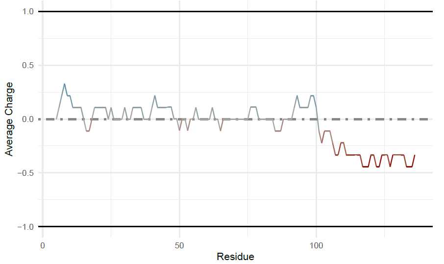
Calculation of Local Charge in alpha−Synuclein.
Window Size = 9 ; Net Charge = −9.048
##
## [[3]]
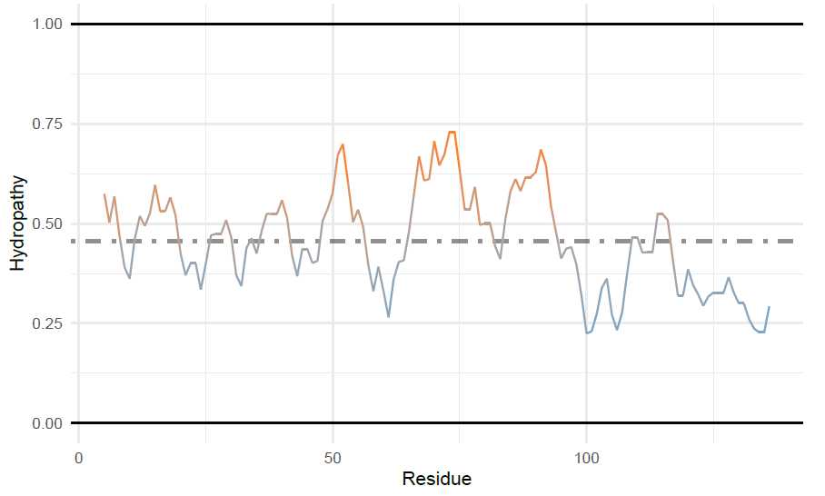
Measurement of Scaled Hydropathy in alpha−Synuclein.
Window Size = 9 ; Average Scaled Hydropathy = 0.455
##
## [[4]]
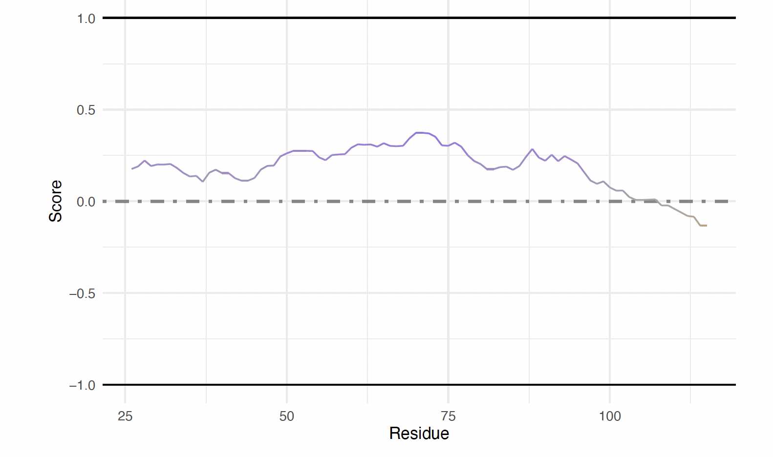
FoldIndex Prediction of Intrinsic Disorder in alpha−Synuclein
##
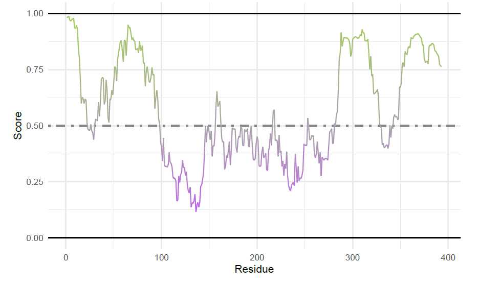
## [[5]]
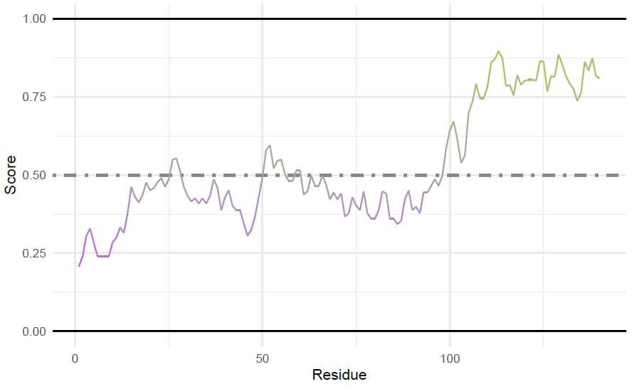
Prediction of Intrinsic Disorder in alpha−Synuclein.
By IUPred2A long
##
## [[6]]
alpha-Synuclein Figures: Generating Supplemental Figures for alpha-Synuclein
The following code generates plots for supplemental figure 1.
Generating Supplemental Figures for alpha-Synuclein: Charge-Hydropathy plot of protein domains
To add multiple points to the charge hydropathy plot, first the sequence will be split into the N-term (residues
1-103) and C-term (residues 104-140). To do this, I will use the ‘AAString’ function from Biostrings . For
the split sequences and the full length sequence, the average net charge and the mean scaled hydropathy are
calculated and put into a data frame. These coordinates will be used for adding ggplot2 annotations. Since
idpr depends on both of these packages, they should already be installed.
# --- Load packages
library(ggplot2)
library(Biostrings)
| A | B | C | D |
|---|---|---|---|
| R | H | Name | Name_Expression |
| 0.047803 | 0.495049 | 1-103 | aSyn [1-103] |
| -0.37783 | 0.34473 | 104-140 | aSyn [104-140] |
| -0.06463 | 0.455321 | 1-140 | aSyn [1-140] |
Then, the ggplot is made and annotations are added. See ggplot2 for annotation options.
# --- Make the base plot
a_syn_split_plot <- chargeHydropathyPlot(a_syn_seq_split)

# --- Add arrows to plot using ggplot2 geom_segment() function.
    # Arrows start at aSyn [1-140] and point to domains.
a_syn_split_plot <- a_syn_split_plot +
    geom_segment(aes(x = 0.4553214, y = -0.06462863, xend = 0.488, yend = 0.03),
                  arrow = arrow(length = unit(0.2, "cm"),
                                type = "closed"))+
    geom_segment(aes(x = 0.4553214, y = -0.06462863, xend = 0.355, yend = -0.358),
                  arrow = arrow(length = unit(0.2, "cm"),
                                type = "closed"))
# --- Add labels to points with ggplot2 functions
a_syn_split_plot <- a_syn_split_plot +
    geom_text(data = RH_DF,
               aes(x = H,
                   y = R,
                   label = Name),
                nudge_x = c(0.05, -0.05, 0.05),
                nudge_y = c(0.07, 0.070, -0.055)
    )
# --- Adds colored points to plot. Adds on top of geom_segment.
a_syn_split_plot <- a_syn_split_plot +
    geom_point(data = RH_DF,
               aes(x = H,
                   y = R),
               color = c("#348AA7", "#92140C", "chocolate1"))
plot(a_syn_split_plot)
```<img src="https://static.yanyin.tech/literature_test/protocol_io_true/protocols.io.b58gq9tw/g2ktbn3x77.jpg" alt="" loading="lazy" title=""/>
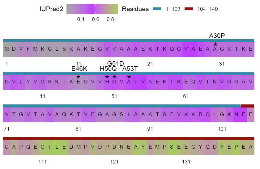
Generating Supplemental Figures for alpha-Synuclein: Sequence Map showing Familial Mutations
Several point mutations in the alpha-Synuclein NTD have been identified that are linked to familial parkinsons disease. These are annotated here in the context of intrinsic disorder predictions from IUPred2. Functions from ggplot2 are needed for annotations, and therefore this package must be attached if not already.
First, the data is retrieved from IUPred2. Setting plotResults = FALSE returns a data frame for custom
plotting.
| A | B | C |
|---|---|---|
| Position | AA | IUPred2 |
| 1 | M | 0.206376 |
| 2 | D | 0.239899 |
| 3 | V | 0.30533 |
| 4 | F | 0.328603 |
| 5 | M | 0.281712 |
| 6 | K | 0.239899 |
Then, a sequence map is created with the IUPred results. Column 2 (a_syn_iupred_df$AA) is a character
vector of individual, single-letter amino acids. Column 3 (a_syn_iupred_df$IUPred2) is a numeric vector
of IUPred2 scores.
iupred_map <-
    sequenceMap(sequence = a_syn_iupred_df$AA,
            property = a_syn_iupred_df$IUPred2,
            nbResidues = 35,
            customColors = c("darkolivegreen3", "grey65", "darkorchid1"))
# --- Plot the unedited, unannotated sequenceMap
plot(iupred_map)
```<img src="https://static.yanyin.tech/literature_test/protocol_io_true/protocols.io.b58gq9tw/g2kxbn3x78.jpg" alt="" loading="lazy" title=""/>
For adding annotations to a sequence map, you can get the position within the plot using the idpr function
‘sequenceMapCoordinates’. This helps guide or identify the coordinates for ggplot2 annotations.
| A | B | C | D |
|---|---|---|---|
| Position | AA | row | col |
| 1 | M | 4 | 1 |
| 2 | D | 4 | 2 |
| 3 | V | 4 | 3 |
| 4 | F | 4 | 4 |
| 5 | M | 4 | 5 |
| 6 | K | 4 | 6 |
Additionally, several annotations are added and the plot themes are edited. See code for all annotations.
Adding the labels for Familial Mutations and ‘*’ to add above the mutated residues. These positions are
determined by ‘sequenceMapCoordinates’ and values are added to row (y) value to move annotations above
letters. To center residues, the column (x) values were adjusted by 0.5 or 0.35.
iupred_map <- iupred_map +
    annotate("text",
             x = c(15.5, 18.5, 30.5, 11.5, 16.5),
             y = c(3.15, 3.15, 4.15, 3.15, 3.3),
             label = c("H50Q", "A53T", "A30P", "E46K", "G51D")) +
annotate("text",
         x = c(15.35, 18.35, 30.25, 11.35, 16.35),
         y = c(2.825, 2.825, 3.825, 2.825, 2.825),
         label = rep("*", 5),
         size = 7)
Finally, the annotated sequence map is plotted.
plot(iupred_map)
Sequence Map of IUPred2 Predictions for aSyn
p53 Figures: Fetching the amino acid sequence
First, I will use the UniprotR package to get the p53 amino acid sequence from the UniProtID. For p53,
the ID is P04637.
## Please wait we are processing your accessions ...
Retrieved Sequence:
print(p53_seq)

## [1] "MEEPQSDPSVEPPLSQETFSDLWKLLPENNVLSPLPSQAMDDLMLSPDDIEQWFTEDPGPDEAPRMPEAAPPVAPAPAAPTPAAPAPAPSWPLSSSVPSQKTYQGSYGFRLGFLHSGTAKSVTCTYS
p53 Figures: Fetching IUPred2A
To retrieve the IUPred2 long and ANCHOR2 scores, the p53 uniprot is used.
iupredAnchor(uniprotAccession = "P04637",
             proteinName = "p53")
Prediction of Intrinsic Disorder in p53.
By IUPred2A long and ANCHOR2
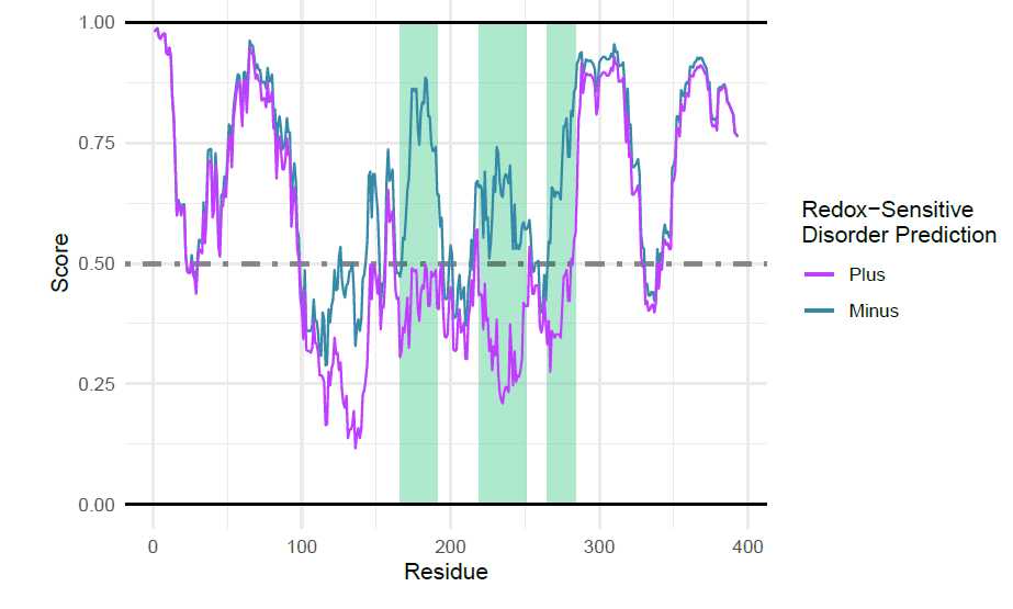
p53 Figures: Fetching IUPred2 Redox
To retrieve the IUPred2 with redox predictions, the p53 uniprot is used.
iupredRedox(uniprotAccession = "P04637",
            proteinName = "p53")
Prediction of Intrinsic Disorder in p53
By IUPred2 long|Based on Environmental Redox State
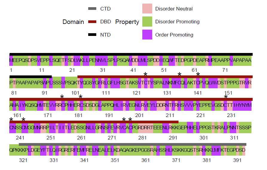
p53 Figures: Making the sequenceMap of p53’s sequence structural tendency
First, the characteristic to map in the plot must be calculated. Here, the tendency for each residue to favor
ordered/disordered structures is determined
tendency_DF <- structuralTendency(p53_seq)
knitr::kable(head(tendency_DF))
| A | B | C |
|---|---|---|
| Position | AA | Tendency |
| 1 | M | Order Promoting |
| 2 | E | Disorder Promoting |
| 3 | E | Disorder Promoting |
| 4 | P | Disorder Promoting |
| 5 | Q | Disorder Promoting |
| 6 | S | Disorder Promoting |
Then, the sequenceMap is made. Since p53 is a long sequence, the nbResidues are increased in the sequenceMap
for easier viewing.
tendency_map <-
    sequenceMap(sequence = tendency_DF$AA,
            property = tendency_DF$Tendency,
            nbResidues = 79,
            customColors = c("#F0B5B3", "darkolivegreen3", "darkorchid1")
            )
plot(tendency_map) #Return the unedited map
```<img src="https://static.yanyin.tech/literature_test/protocol_io_true/protocols.io.b58gq9tw/g2mfbn3x712.jpg" alt="" loading="lazy" title=""/>
To get the coordinates for ggplot annotations, the ‘sequenceMapCoordinates’ function can assist. Since the
default has been changed for nbResidues, from 30 to 79, this must change in the coordinates function to
properly calculate the position of each residue within the sequenceMap.
p53_coords <- sequenceMapCoordinates(p53_seq,
                        nbResidues = 79)
knitr::kable(head(p53_coords)) #Top of results to show example
| A | B | C | D |
|---|---|---|---|
| Position | AA | row | col |
| 1 | M | 5 | 1 |
| 2 | E | 5 | 2 |
| 3 | E | 5 | 3 |
| 4 | P | 5 | 4 |
| 5 | Q | 5 | 5 |
| 6 | S | 5 | 6 |
Additional annotations are made, see the code and the example from Fig. S1B on working with sequenceMap
and annotations.
After annotations and titles have been added, the plot can be generated.
plot(tendency_map)
Sequence Map of Residue Tendency for p53.
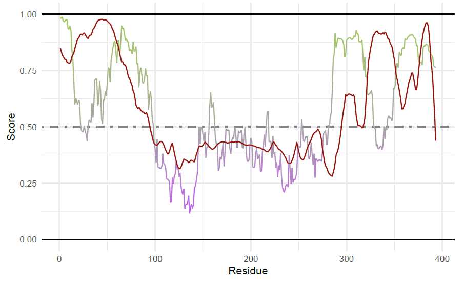
p53 Figures: Generating the idprofile for p53
To get the ‘idprofile’, a simple function is needed with the sequence and Uniprot ID specified. This generates
all plots in supplementary figure 2.
idprofile(sequence = p53_seq,
          uniprotAccession = "P04637",
          proteinName = "p53") #Specifying proteinName automatically names plot
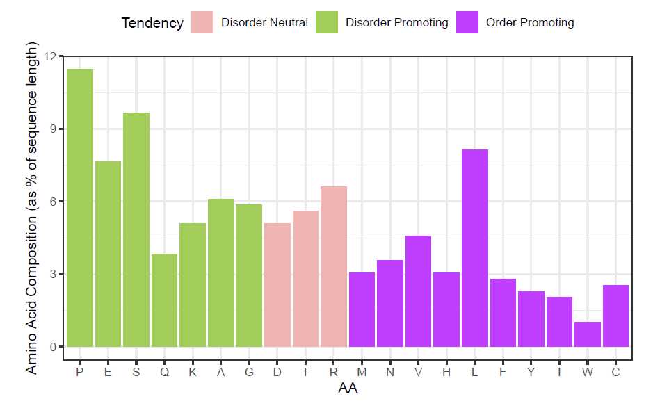
## [[1]]
```<img src="https://static.yanyin.tech/literature_test/protocol_io_true/protocols.io.b58gq9tw/g2nbbrwd718.jpg" alt="" loading="lazy" title=""/>
Compositional Profile of p53
##
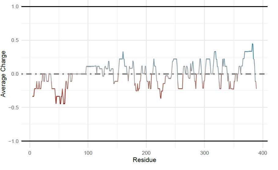
## [[2]]
Calculation of Local Charge in p53
Window Size = 9 ; Net Charge = −5.774
##
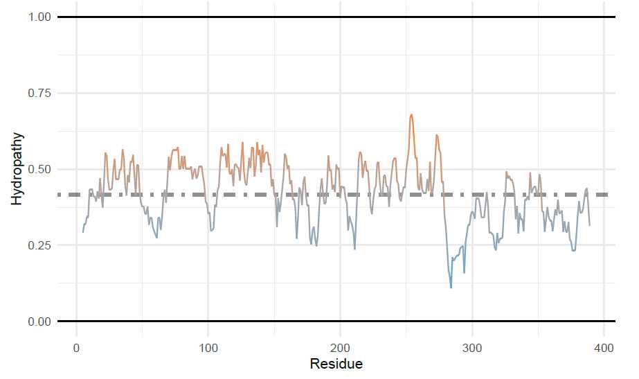
## [[3]]
Measurement of Scaled Hydropathy in p53
Window Size = 9 ; Average Scaled Hydropathy = 0.416
##
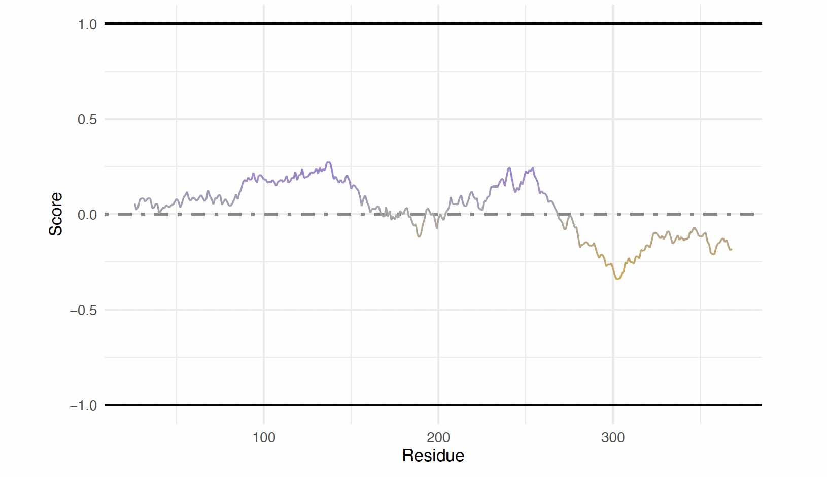
## [[4]]
FoldIndex Prediction of Intrinsic Disorder in p53
##
## [[5]]
Prediction of Intrinsic Disorder in p53
By IUPred2A long
##
## [[6]]
