Spooling electrochemiluminescence spectroscopy: development, applications and beyond
Mahdi Hesari, Zhifeng Ding
Electrochemiluminescence
Spooling Spectroscopy
Light Generation Mechanism
Electron Transfer Pathways
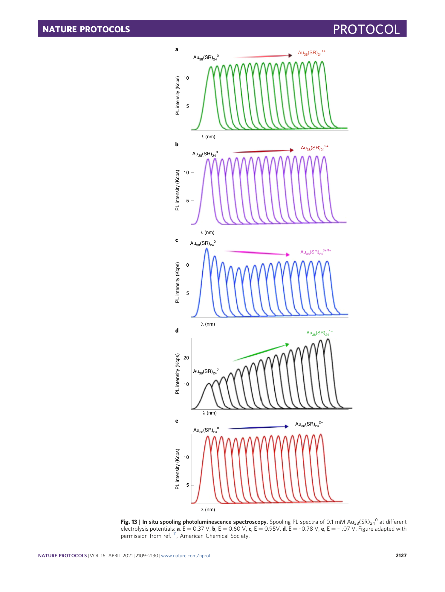
Spooling Photoluminescence


Extended
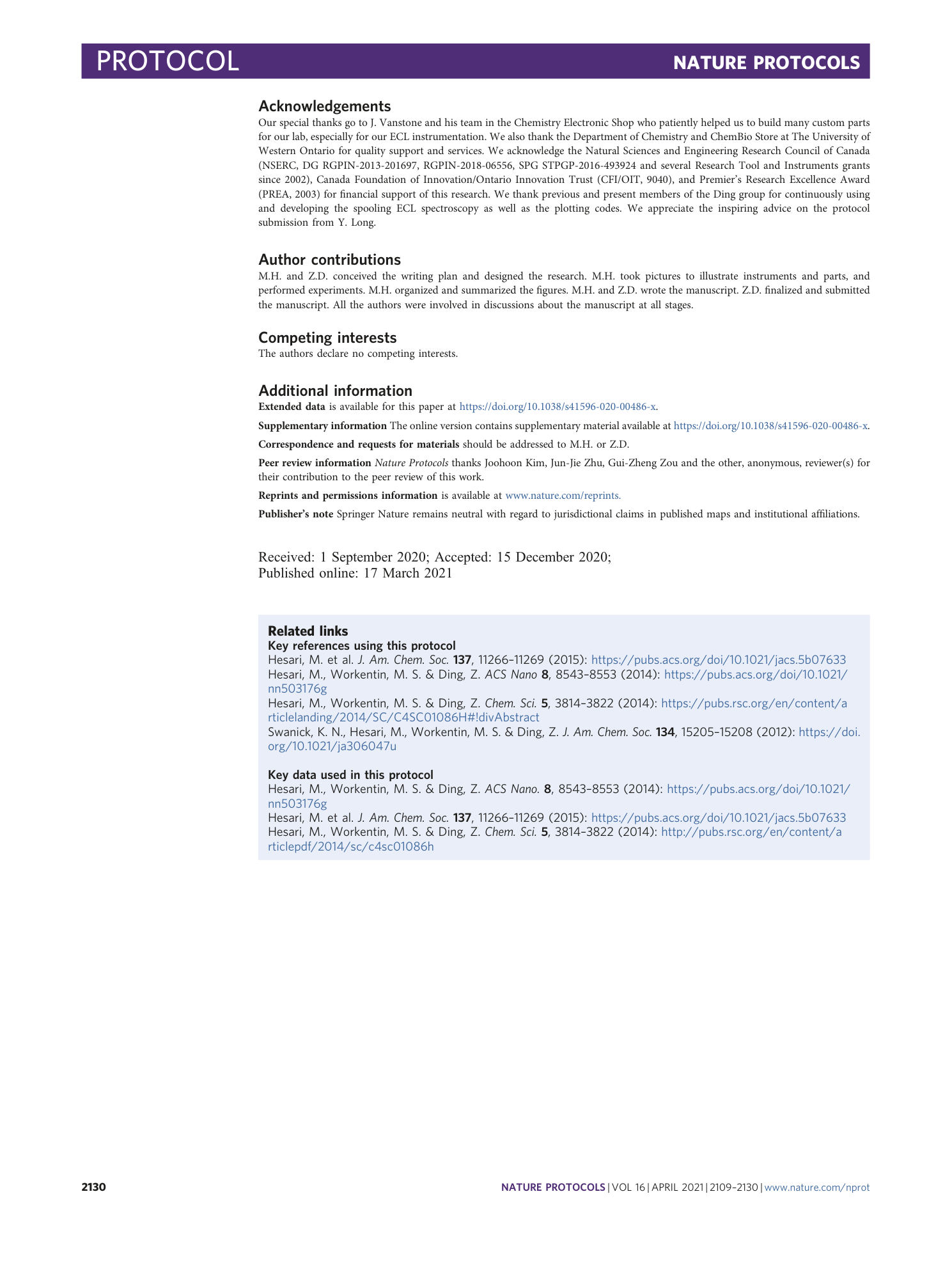
Extended Data Fig. 1 Assembly of a platinum electrode inside a soft glass.
A vacuum tube is attached to one end of the soft glass to assist with Pt rod insertion into the other end.
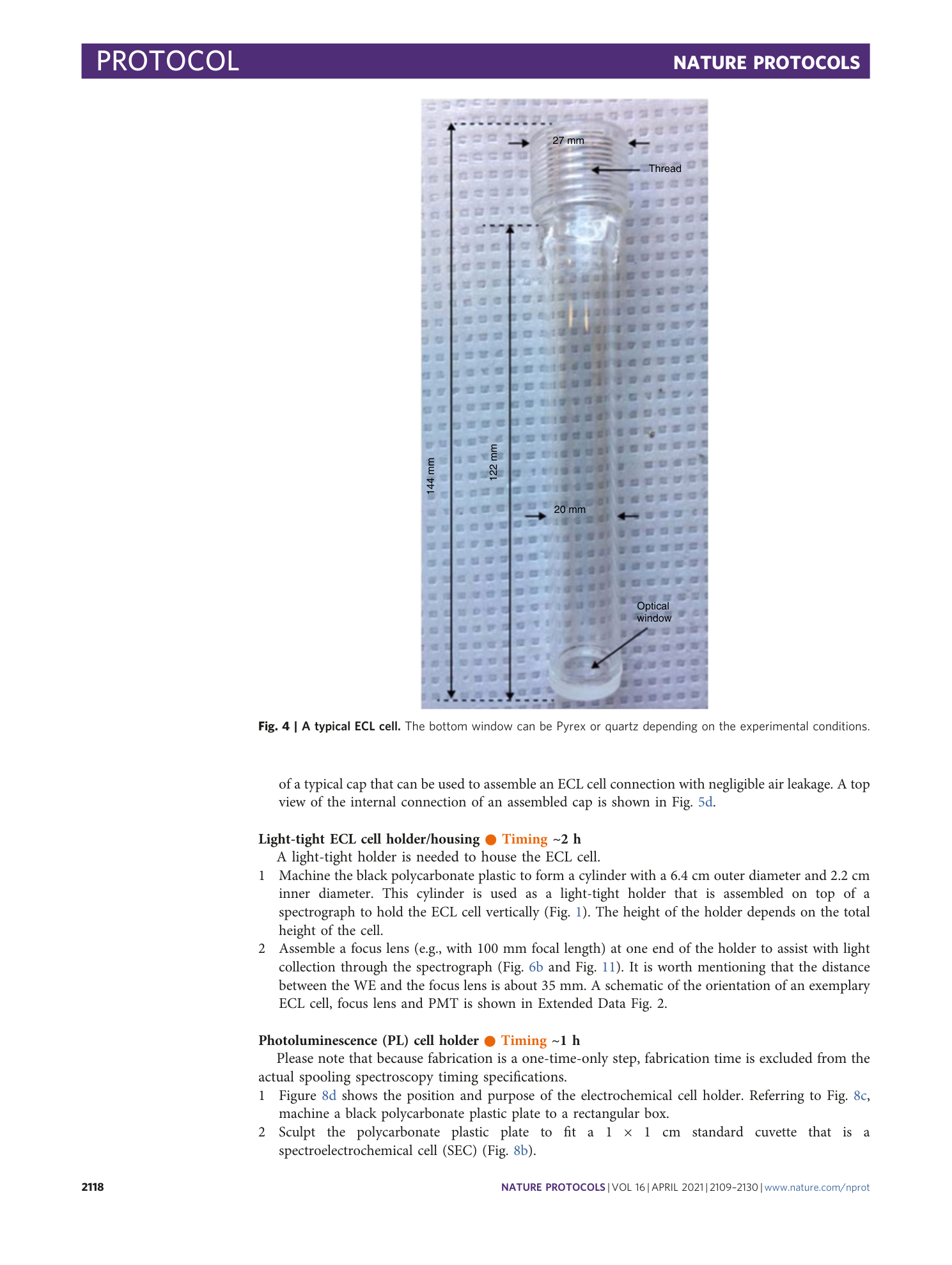
Extended Data Fig. 2 Schematic assembly of ECL cell-focus lens-PMT.
A photograph of an exemplary ECL cell including WE (Pt disc), CE (Pt coil), RE (Pt coil), sample solution, quartz window, focus lens, and a PMT along with a recorder. Note that the represented distances are not scaled.
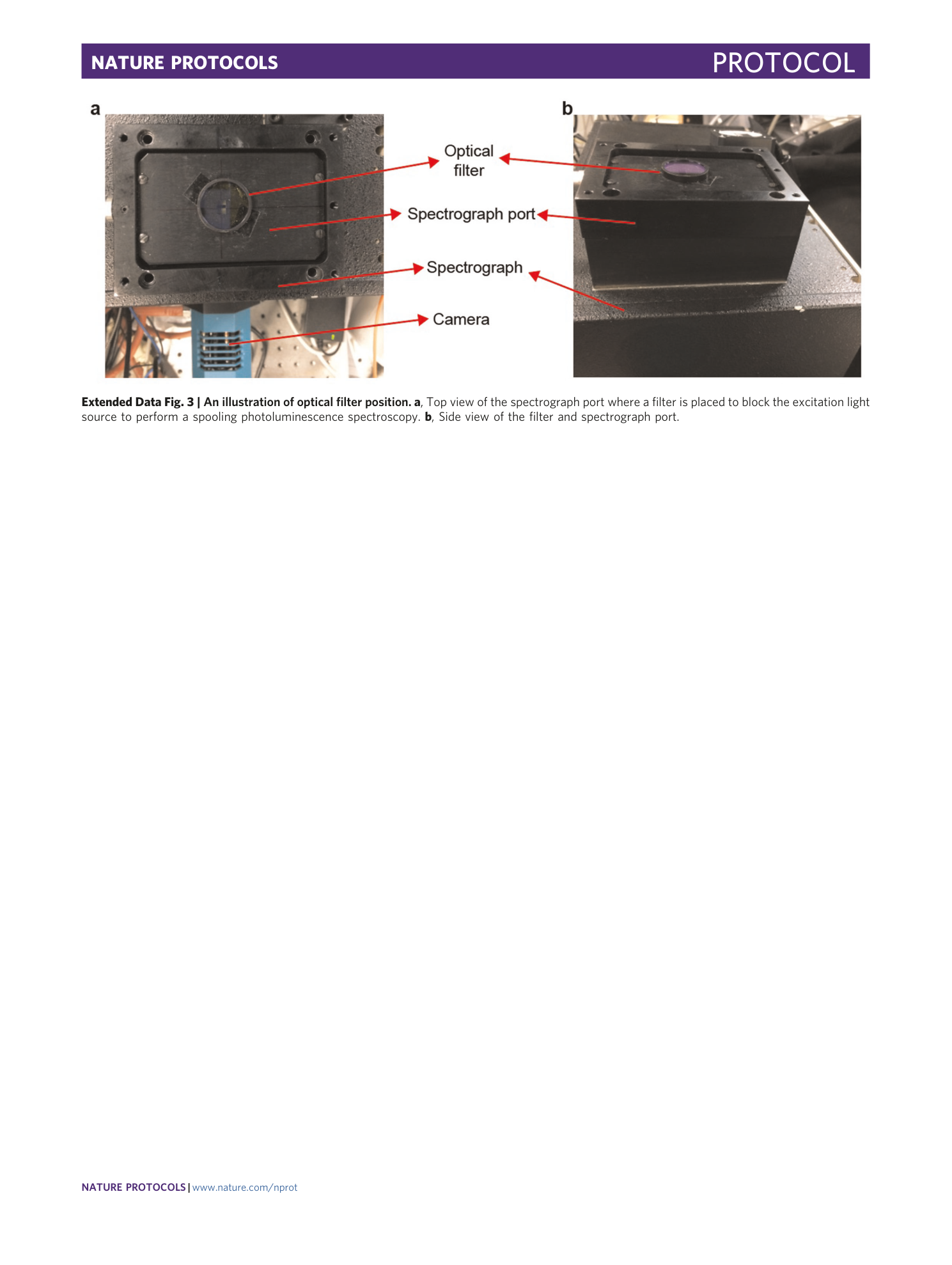
Extended Data Fig. 3 An illustration of optical filter position.
a , Top view of the spectrograph port where a filter is placed to block the excitation light source to perform a spooling photoluminescence spectroscopy. b , Side view of the filter and spectrograph port.
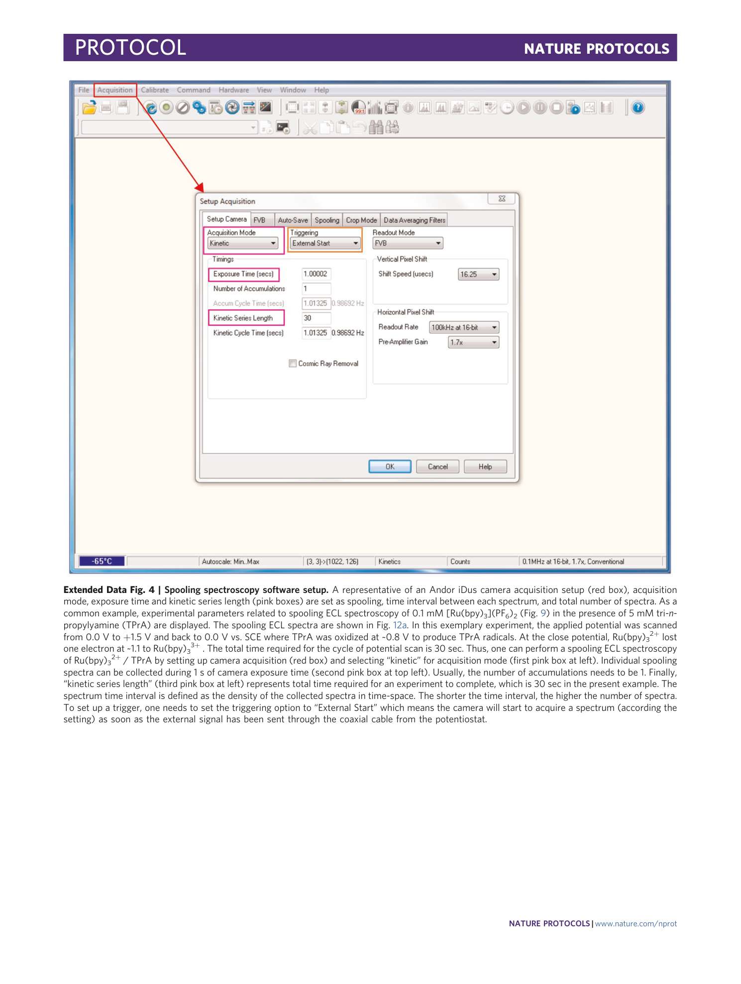
Extended Data Fig. 4 Spooling spectroscopy software setup.
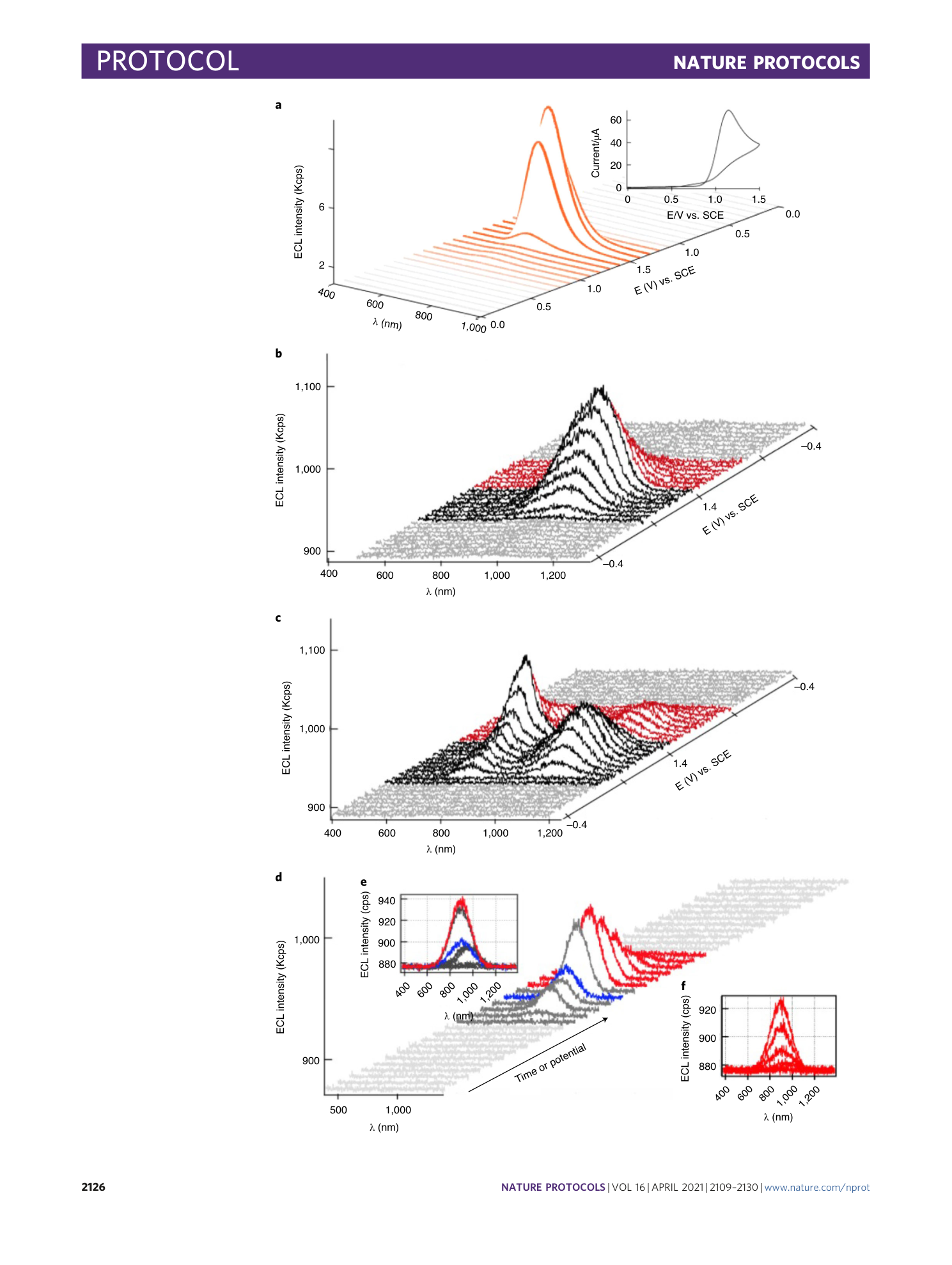
A representative of an Andor iDus camera acquisition setup (red box), acquisition mode, exposure time and kinetic series length (pink boxes) are set as spooling, time interval between each spectrum, and total number of spectra. As a common example, experimental parameters related to spooling ECL spectroscopy of 0.1 mM [Ru(bpy) 3 ](PF 6 ) 2 (Fig. 9 ) in the presence of 5 mM tri- n -propylyamine (TPrA) are displayed. The spooling ECL spectra are shown in Fig. 12a . In this exemplary experiment, the applied potential was scanned from 0.0 V to +1.5 V and back to 0.0 V vs. SCE where TPrA was oxidized at ~0.8 V to produce TPrA radicals. At the close potential, Ru(bpy) 3 2+ lost one electron at ~1.1 to Ru(bpy) 3 3+ . The total time required for the cycle of potential scan is 30 sec. Thus, one can perform a spooling ECL spectroscopy of Ru(bpy) 3 2+ / TPrA by setting up camera acquisition (red box) and selecting “kinetic” for acquisition mode (first pink box at left). Individual spooling spectra can be collected during 1 s of camera exposure time (second pink box at top left). Usually, the number of accumulations needs to be 1. Finally, “kinetic series length” (third pink box at left) represents total time required for an experiment to complete, which is 30 sec in the present example. The spectrum time interval is defined as the density of the collected spectra in time-space. The shorter the time interval, the higher the number of spectra. To set up a trigger, one needs to set the triggering option to “External Start” which means the camera will start to acquire a spectrum (according the setting) as soon as the external signal has been sent through the coaxial cable from the potentiostat.
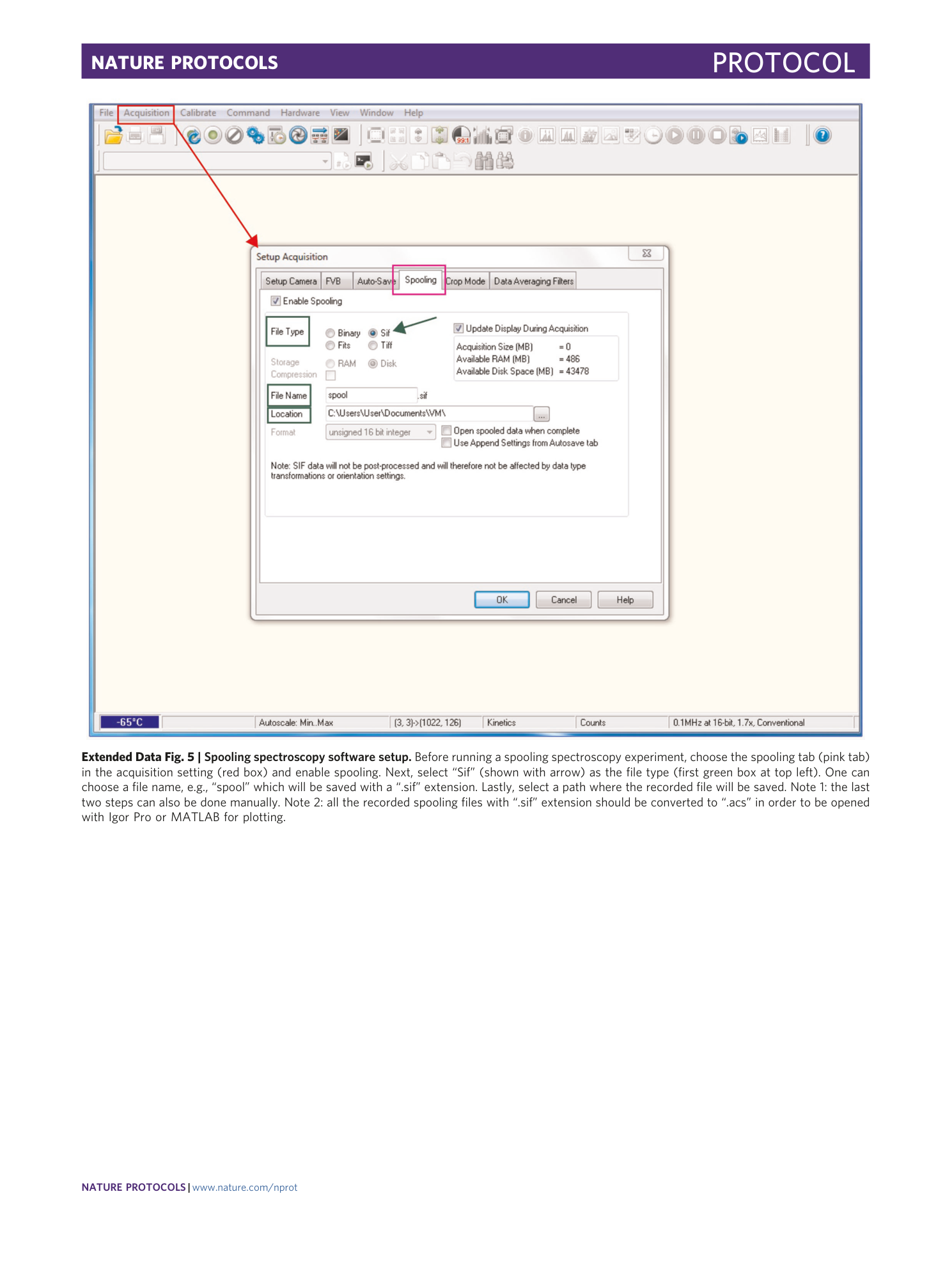
Extended Data Fig. 5 Spooling spectroscopy software setup.
Before running a spooling spectroscopy experiment, choose the spooling tab (pink tab) in the acquisition setting (red box) and enable spooling. Next, select “Sif” (shown with arrow) as the file type (first green box at top left). One can choose a file name, e.g., “spool” which will be saved with a “.sif” extension. Lastly, select a path where the recorded file will be saved. Note 1: the last two steps can also be done manually. Note 2: all the recorded spooling files with “.sif” extension should be converted to “.acs” in order to be opened with Igor Pro or MATLAB for plotting.
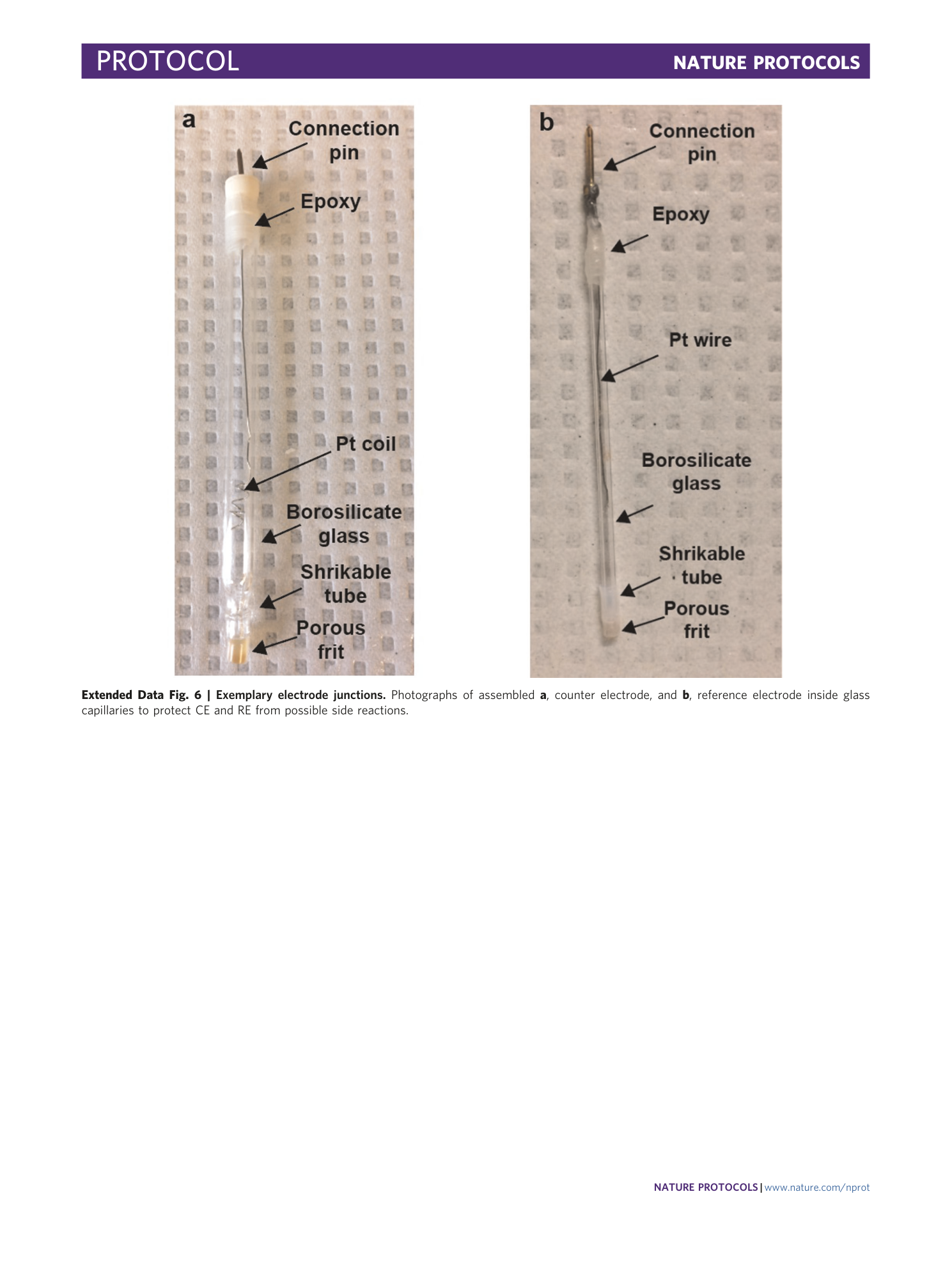
Extended Data Fig. 6 Exemplary electrode junctions.
Photographs of assembled a , counter electrode, and b , reference electrode inside glass capillaries to protect CE and RE from possible side reactions.
Supplementary information
Reporting Summary
Supplementary Data 1
Manual to use spooling spectroscopy of Ru(bpy) with TPrA and sample spooling ECL plot using MATLAB software.
