QUINT Workflow for Fluorescence

Open the QuPath application. Select ‘Create project’.

Select your slide/stain folder within your QUINT Workflow project folder (i.e., slide24stain19).

Select ‘Add images’ > ‘Choose files’. Navigate to the image file and select ‘Open’. Set image type to Fluorescence. Select ‘Import’.

Double click on the first image for it to appear in the viewing window.

Open the Brightness & contrast window (

) and leave it open.

Select ‘Automate’ > ‘Show script editor’. Run the following script (change the channel names to the corresponding channels for your stain). This will change your channel names to the appropriate names.

Stay on the first image. In the script editor window select ‘Run’ > ‘Run for project’. Move all the images over to the selected column except for the first image. You cannot run a script for the whole project on an image that you have currently open in the viewer. Select ‘OK’. Close the script editor.

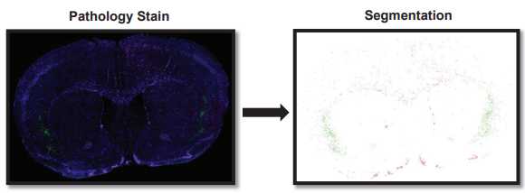
For each image, adjust the Min and Max display in the Brightness & contrast window for each channel as needed to make the scan easier to see. This only changes your visual, no actual properties of the scan. Pathology Stain Segmentation

Create annotation classifications for any new channel names you have previously not worked with. Select the ‘Annotations’ tab > three dots in the bottom right of the window > populate from image channels. Ensure that the class color matches the channel color.

Select the rectangle button (

) and select your ROI around the first brain.

Lock the rectangle by selecting the annotation (the rectangle will appear yellow). Right click inside the rectangle, select ‘Annotations’ > ‘Lock’. This will lock the rectangle, so it is not accidentally moved.

MAKE SURE THE RECTANGLE IS SELECTED (YELLOW) AS YOU COMPLETE THIS STEP. Select ‘File’ > ‘Export Images’ > ‘Rendered RBG (with overlays)’. Set the export format to (PNG). Set the downsample factor to 12.0. Select OK.

Save in the QVN folder with the appropriate naming designation (i.e., sl18st3sc1_s041, sl18st3sc2_s042_).

Repeat steps 10-13 for each image.

Select ‘Analyze’ > ‘Cell Detection’ > ‘Cell Detection’ to open the cell detection window.

Adjust the Cell Detection parameters as needed. The most helpful parameters to adjust are Sigma, Minimum Area, Maximum Area, Threshold, and Cell Expansion.

a. Minimum Area and Maximum Area will be dependent on whether you are analyzing mouse or human tissue.

b. Keep all checkboxes checked “Split by Shape”, “Include Cell Nucleus”, “Smooth Boundaries”, and “Make Measurements”.

c. A lower Sigma value will break up nuclei more. A higher Sigma value will combine nuclei more often.

d. Once you are satisfied with the parameters, you can save the Cell Detection script to easily apply it to your other images. The same cell detection parameters must be applied to all images.

Remove cells from areas of damaged tissue or outside the brain.

Select the three dots to the right of ‘Auto Set’ > ‘Add/Remove…’ > ‘Add class’. Name the new class ‘Training’.

Choose 6-7 regions across all 8 images to use as training images. These regions should be ones that contain a variety of staining to properly train the classifier.

For each annotation rectangle created for the training classifier, set its class to ‘Training’ by right clicking in the annotation rectangle > ‘Set class’ > ‘Training’.

Once you have created all your training annotations, select ‘Classify’ > ‘Training images’ > ‘Create training image’. Set the classification of your combined training annotations to ‘Training’ and select ‘Rectangles only’. Set the image type of your combined training annotations to ‘Fluorescence’.

Create a duplicate of the combined training annotations for each different channel you have (excluding your nuclear stain). Rename the image to include the channel name. To duplicate, right click on the combined training annotation image and select ‘Duplicate image(s)’.

Draw a rectangle annotation around each training image. Lock the annotation. Run cell detection with the same parameters as your individual images.

Select ‘Classify’ > ‘Object classification’ > ‘Train object classifier’. Set the object filter to ‘Cells’, the classifier to ‘Artificial neural network (ANN_MLP)’, features to ‘Selected measurements’, classes to ‘All classes’, and training to ‘All annotations’. Select ‘Select’ to the right of ‘Selected measurements’ and select all measurements corresponding to the selected training channel. Leave the window open.

Open the points window (

). Select ‘Add’ two times to add two annotations. Set the first annotation to ‘Ignore*’ by right clicking on the annotation and select ‘Set class’ > ‘Ignore*’. Set the second annotation to the channel you are training.

In the Brightness & contrast window, turn off all channels except the channel you are training.

Train the classifier by using the points annotations to identify cells as either positive for the channel or ignore. Continue training the classifier until you are satisfied with the predicted output. Select live update to view how the points you select are affecting the classifier.

Give the classifier a name with the slide number, stain number, the channel, and the date (i.e., slide24stain19_Nr4a2_12.16.22). Select ‘Save’.

Repeat steps 24-28 for every training image.

Select ‘Classify’ > ‘Object classification’ > ‘Create composite classifier’. Move the individual classifiers to the ‘selected’ side of the window in the order you want them to be applied. Enter a name for the combined classifier (i.e., sl18st19_composite_11.22.22) and select ‘Save & apply’.

For each whole brain image, select ‘Classify’ > ‘Object classification > ‘Load object classifier’, select the composite classifier you just created and ‘Apply classifier’.

To show sub-classes identified from your composite classifier (cells identified as positive for multiple channels) navigate to the ‘Annotations’ tab > three dots button in the bottom right of the window > ‘Populate from existing objects’ > ‘All classes (including sub-classes)’. Select ‘Yes’ when asked if you want to keep the existing available classes.

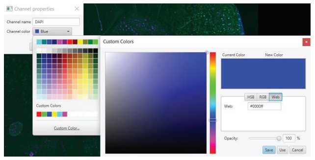
Write down the 6-digit web color code for each sub-class in your annotation window. You will need this information for Nutil. Double click the channels listed in the annotations tab to view the color code.

Navigate to each scene image and rename the annotation that is off the entire brain image. Rename by right-clicking on the selected annotation image > ‘Annotations’ > ‘Set properties’. Rename the annotation using the following naming convention: ‘sl18st19sc1input_s041_’ ; ‘sl18st19sc2input_s042_’.

Navigate to one of your combined training images.

Select ‘Automate’ > ‘Show script editor’.

Enter the script in the blue box below at line 1. You can export multiple cell classifications together to simplify the downstream Nutil input. To do so, add more lines with

“.addLabel(‘Name of classification’, #).

Select ‘Run’ > ‘Run for project’. Move each scene image over to the ‘Selected’ window and select ‘OK’.

import qupath.lib.images.servers.LabeledImageServer 
def imageData = getCurrentImageData() 
// Define output path (relative to project) 
def name = GeneralTools.getNameWithoutExtension(imageData.getServer().getMetadata().getName()) 
def pathOutput = buildFilePath(PROJECT_BASE_DIR, 'export', name) 
mkdirs(pathOutput) 
// Export at full resolution 
double downsample = 1.0 
// Create an ImageServer where the pixels are derived from annotations 
def labelServer = new LabeledImageServer.Builder(imageData) 
 .backgroundLabel(0, ColorTools.WHITE) // Specify background label (usually 0 or 255) 
 .downsample(downsample) // Choose server resolution; this should match the resolution at which tiles are exported 
 .addLabel('Slc17a7', 1) // Choose output labels (the order matters!) 
.addLabel(‘Gad1’, 2) 
 .multichannelOutput(false) // If true, each label refers to the channel of a multichannel binary image (required for multiclass 
probability) 
 .build() 
// Export each region 
int i = 0 
for (annotation in getAnnotationObjects()) { 
 name = annotation.getName() 
 if (annotation.getROI().getRoiName() == "Rectangle") { 
 def region = RegionRequest.createInstance( 
 labelServer.getPath(), downsample, annotation.getROI()) 
 i++ 
 def outputPath = buildFilePath(pathOutput, name + '.png') 
 writeImageRegion(labelServer, region, outputPath) 
}} 

Find the exported images in the export folder. The segmentation image should be white with objects in their WEB ID color. The images should be the exact same dimensions of the earlier region of interest image you created as a PNG with a downsize factor of 12.

Scenes with smaller annotation regions that you used to make your training images will have a second segmentation. Delete the segmentation image that corresponds to the smaller annotation.

Copy the images to the ‘Input’ folder in the QVN folder. These images will be used in the final step of Nutil. Close the QuPath application.

Open the QuickNII program folder.

Open Filebuilder .

Navigate to the QVN folder with the brain image exports from QuPath. These images are not the segmentation exports, but the original brain image exports. These images must all be surrounded by a yellow rectangle.

Select all the images to be registered and select ‘Open’. It is useful to add a shortcut of your QUINT Workflow folder to your desktop for simpler navigation.

Select ‘Save XML’. Navigate to the QVN folder and save as ‘Filebuilder XML’. Make sure to save this file in the same folder as the brain image exports from QuPath.

Close Filebuilder.

Open the QuickNII application. Select ‘Manage data’ > ‘Load’ and select the XML file that was just generated in step 5.

Double click on the first image in Filebuilder to have it show up in the viewing window in the QuickNII application.

Select ‘Rainbow 2017’ from the drop-down menu in the upper left-hand corner of the toolbar (1).

You can adjust how you see the atlas overlay by dragging the vertical transparency bar on the left side of the screen (2).

For the first section, find the anteroposterior position. To do this, drag the sagittal red dot (3) to the correct rostro-caudal position. Select ‘Store’ to save the position.

Repeat step 11 for the last section. This will bring all other sections to the approximately correct position.

Adjust each individual section to the appropriate place in the atlas. Many adjustments may need to be made until the correct plane of section is identified.

a.  **Rotation** : clockwise or counterclockwise (4).

b. **Brain size** e: in the x and y direction (5). 

c **Rostro-caudal position** on: adjust sagittal view. 

 **Left-right plane** ane: adjust horizontal view. 

**Front-back plane** lane: adjust sagittal view.

Select ‘Store’ before moving off a section or it will not save!

Navigate to the next section by double clicking on the section in the Filebuilder, or by selecting the arrows in the upper-right corner. Edit all sections as noted in step 13.

Select ‘Manage data’ > ‘Export Propagation’ and save this XML filed as “QuickN XML.xml” within the QVN folder. It is not automatically recognized as a .xml file, hence the need to add “.xml” to the end of the name.

Select ‘Save JSON’ and name it “QuickN JSON” within the QVN folder. This JSON file is used for VisuAlign. Make sure to save the JSON file in the same folder as the brain image exports from QuPath and the Filebuilder XML file.

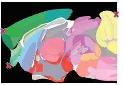
In the QuickNII application, go back to the first section. Show just the rainbow atlas image.

Adjust the horizontal plane to a hemispheric split (completely vertical). Ensure proper bisecting by confirming it within the coronal plane. You want to perfectly bisect the coronal plan. Change the angle if needed.

Hover the cursor over the brain viewing window and record the x-y-z coordinates (shown in the top left of the window) for the following three parts of the brain: top left, top right, and bottom left.

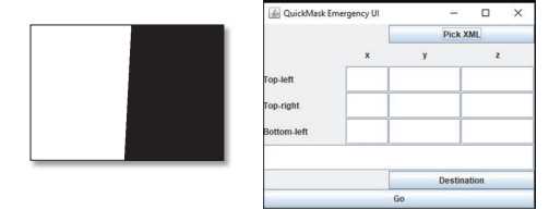
Open the QMask tool and select ‘Pick XML’ and open the QuickN XML file generated in QuickNII.

Enter the x-y-z coordinates.

Select ‘Destination’ and navigate to the Mask folder within your current project folder and select ‘Open’.

Select ‘Go’. The mask output should be a black and white PNG. Close QuickNII and the QMask tool.

Ensure the mask files are named using the appropriate naming convention (i.e., sl18st3sc1_s041_mask).

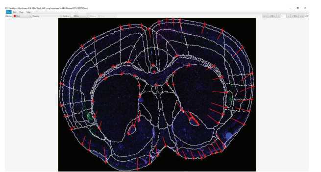
You can check to see if your mask outputs accurately bisect for a hemispheric split by comparing the mask output to the output from VisuAlign.

Open the VisuAlign application.

Select ‘File’ > ‘Open’ and select the QuickN JSON file you created in QuickNII.

Drag the opacity bar all the way to the right towards ‘Outline’. This will display an outline of all the regions. This is the easiest format for transformation. You can change the color of the outline and the marker for easier visualization.

Align all regions properly.

Hover over an atlas region.

To create a marker, click the space bar.

Drag the maker symbol to the correct location.

Markers can be moved at any point. To delete a maker, hover over the maker and click delete on the keyboard.

Markers can be moved at any point. To delete a maker, hover over the maker and click delete on the keyboard.

Select the < and > arrows at the top-right to navigate between sections. There is no need to save

or store these as in QuickNII.

Once all images are complete, select ‘File’ > ‘Save as’ and save as ‘VisuAlign JSON’ in the QVN folder. This can be opened again to continue aligning later.

Select ‘File’ > ‘Export’ and navigate to the Atlas folder and select ‘Select Folder’. This will export the files needed for Nutil . These are also the images that you can compare to the Mask outputs to determine the accuracy of your hemispheric split.

Open the Nutil application and navigate to the ‘Operation’ tab.

Select ‘New’. Select ‘Quantifier’ from the drop-down menu and select ‘Ok’.

Select ‘Save’ to save the overall Nutil project (i.e., “sl24st19.nut”).

Name each project using the following naming convention: ‘sl#st#_classifier_left/right’.

Set the ‘Segmentation folder’ to the ‘Input’ folder within the QVN folder.

Set the ‘Brain atlas map folder’ to the ‘Atlas’ folder within the QVN folder.

Select ‘Reference atlas’ to the ‘Allen Mouse Brain 2017’.

Set the ‘XML or JSON anchoring file’ to the ‘VisuAlign JSON.json’ file.

Set the ‘Output folder’ to the ‘Output_left’ or ‘Output_right’ folder within the QVN folder depending on which hemisphere you are running.