Analytical Workflows for Single-Cell Multiomic Data Using the BD Rhapsody Platform

Wenyan Li, Wenyan Li, Sajad Razavi Bazaz, Sajad Razavi Bazaz, Chelsea Mayoh, Chelsea Mayoh, Robert Salomon, Robert Salomon

Published: 2024-02-14 DOI: 10.1002/cpz1.963

Abstract

The conversion of raw sequencing reads to biologically relevant data in high-throughput single-cell RNA sequencing experiments is a complex and involved process. Drawing meaning from thousands of individual cells to provide biological insight requires ensuring not only that the data are of the highest quality but also that the signal can be separated from noise. In this article, we describe a detailed analytical workflow, including six pipelines, that allows high-quality data analysis in single-cell multiomics. © 2024 The Authors. Current Protocols published by Wiley Periodicals LLC.

Basic Protocol 1 : Image analysis

Basic Protocol 2 : Sequencing quality control and generation of a gene expression matrix

Basic Protocol 3 : Gene expression matrix data pre-processing and analysis

Basic Protocol 4 : Advanced analysis

Basic Protocol 5 : Conversion to flow cytometry standard (FCS) format

Basic Protocol 6 : Visualization using graphical interfaces

INTRODUCTION

Since the advent of high-throughput single-cell genomic approaches in 2015 (Klein et al., 2015; Macosko et al., 2015), cytometry has seen a rapid expansion in the availability of high-dimensional single-cell characterization tools. Single-cell RNA sequencing (scRNA-seq) (Buenrostro et al., 2015; Rotem et al., 2015), single-cell DNA sequencing (Pellegrino et al., 2018), single-cell epigenetic analysis (Macaulay et al., 2015), high-dimensional characterization of cell surface proteins (Shahi et al., 2017), and combinations of these approaches (Peterson et al., 2017; Shahi et al., 2017; Stoeckius et al., 2017) are providing new insights into biology and disease at single-cell resolution. Although commonly referred to as single-cell genomics, some have argued that genomic cytometry may be a more apt description, as these approaches aim to characterize and measure cells (cytometry) rather than focusing on their genomic profiles (Salomon et al., 2020). This is exemplified by approaches such as CITE-seq, REAP-Seq, and AbSeq (Peterson et al., 2017; Shahi et al., 2017; Stoeckius et al., 2017) that use genomic readouts to study protein expression and are not restricted to measuring the genomic characteristics of the cells.

Single-cell genomics and genomic cytometry approaches have allowed biologists to study cells and cellular machinery in unprecedented detail. Before 2015, single-cell analysis was generally limited to a few markers or a restricted number of cells; however, advances in genomics, coupled with the decreasing cost of sequencing, have provided the potential to look at thousands of target molecules in thousands of cells simultaneously. This is particularly the case for scRNA-seq, where whole transcriptome analysis (WTA) typically gives 3000 to 5000 transcripts per cell, and for oligo antibody approaches, where hundreds of cell surface proteins can be simultaneously analyzed (Wu, Al-Eryani et al., 2021).

From a biological perspective, single-cell genomics and genomic cytometry have been used to discover new cell types in complex tissue such as the brain (Hodge et al., 2019), blood (Chen et al., 2022; Lawlor et al., 2021), and eye (Collin et al., 2021; Lukowski et al., 2019; Macosko et al., 2015). In addition, these approaches have been used to study disease progression in conditions such as cancer (Song et al., 2022; Valdés-Mora et al., 2021; Wu, Fan et al., 2021), diabetes (Wilson et al., 2019), and COVID-19 (Speranza et al., 2021; Zhu et al., 2020). They have also been applied to understand normal developmental processes (Briggs et al., 2018; Cao et al., 2019; Farrell et al., 2018; Wagner et al., 2018).

The most popular single-cell characterization approach is scRNA-seq using the Chromium 10× system for cell capture and library preparation coupled with Cell Ranger for demultiplexing and alignment, followed by use of Seurat (Hao et al., 2021) for data analysis. However, as the field matures, more systems and approaches are becoming available. One such system is the BD Rhapsody. Unlike the well-documented and abundant vignettes for the Chromium 10×, papers describing the analysis of BD Rhapsody data are limited.

Based on the Seq-Well protocol (Gierahn et al., 2017), the BD Rhapsody system uses microfluidic chips consisting of about 240,000 microwells to create a plate array where cells can be captured and lysed in the presence of beads coated in oligos containing a poly T region, cell-specific barcode, and unique molecular identifier (UMI) and unique sequence regions that facilitate molecular amplification. The workflow of scRNA-seq using the BD Rhapsody system is illustrated in Figure 1.

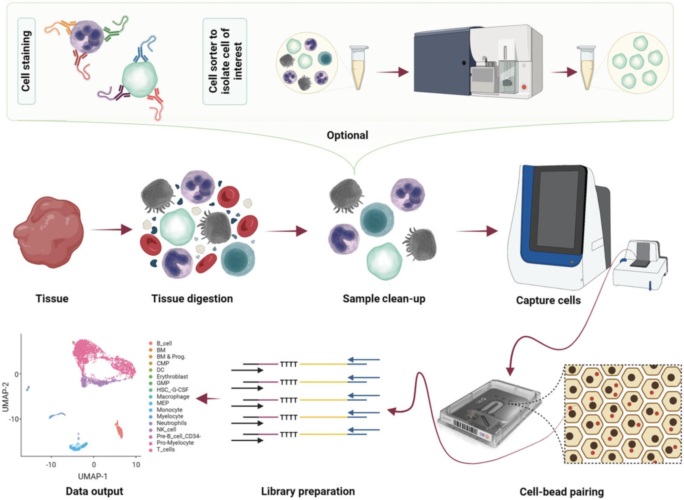
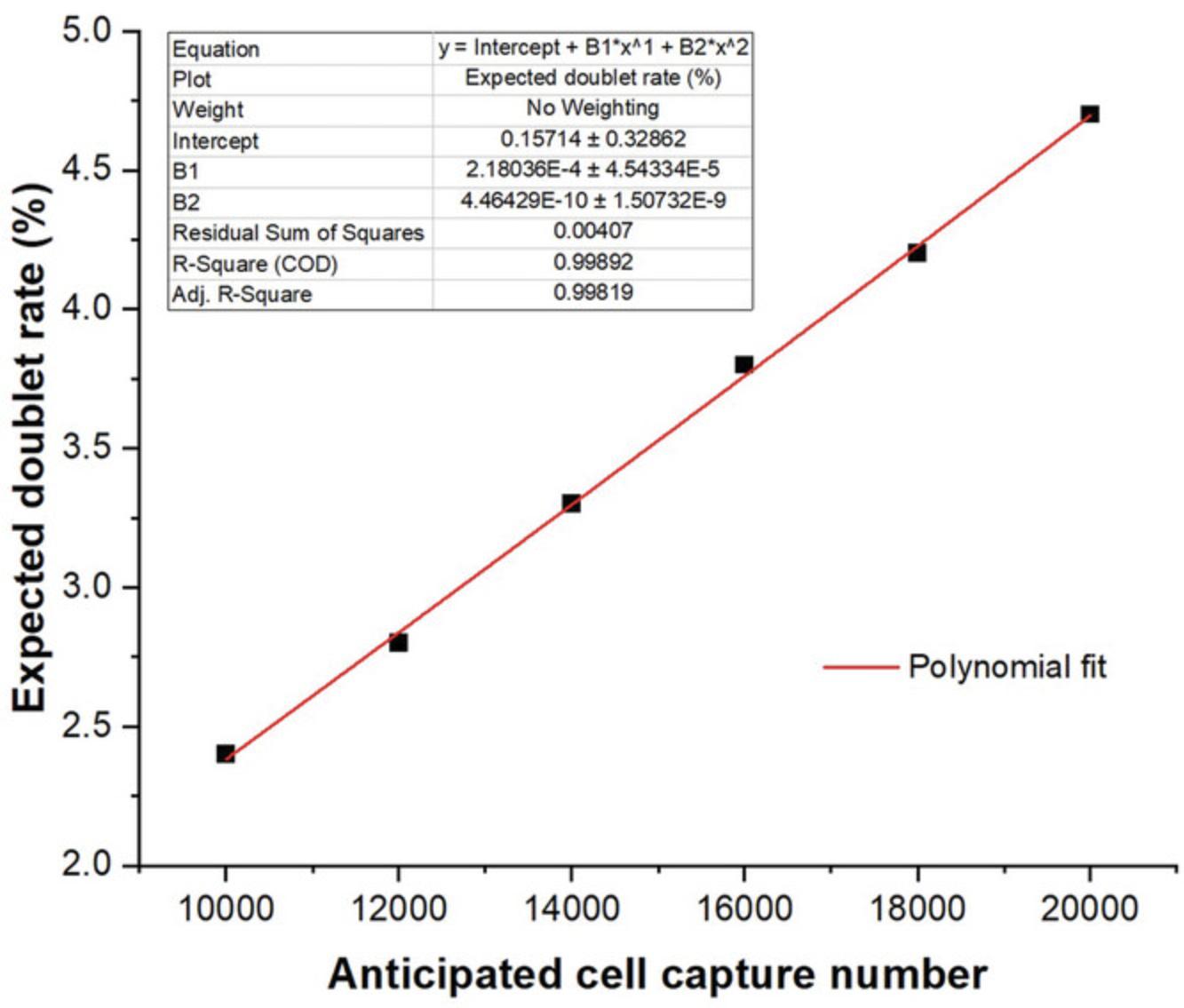
BD Rhapsody–based workflows for obtaining high-quality scRNA-seq data. If using solid tissue, digestion must precede sample clean-up prior to loading into the BD Rhapsody capture workflows. Sample clean-up is critical and may involve an optional cell staining and sorting step. Once the cell sample is prepared, it can be loaded into the BD Rhapsody to pair a cell with a polyadenylated paramagnetic bead containing a unique cellular barcode. Following the cell-bead pairing, a sequencing library is created, the library is sequenced, and the data can be analyzed.

The BD Rhapsody is unique from the Chromium 10× as it does not use water-in-oil droplets (reducing the instability associated with droplet microfluidics), uses hard magnetic capture beads rather than dissolvable GEMS (providing easy cell number subletting and allowing cDNA to be retained on a per-cell basis), involves multiple imaging steps during the capture process (see discussion below), and has significantly lower doublet rates at the same cell capture numbers (Fig. 2).

Anticipated doublet rates based on cell capture numbers in the BD Rhapsody platform.

This imaging step is particularly useful when processing clinical samples as it 1) accurately determines doublet rates, not relying on cell mixing experiments to determine theoretical doublet rates and giving accurate doublet rates for each individual experiment; 2) quantifies cell viability (through Calcein AM positivity and DRAQ7 negativity); 3) visualizes basic cell properties, such as size; 4) provides valuable image-based quality control (QC) checkpoints to monitor each of the main cell capture steps; and 5) allows visualization of potential clusters.

An important molecular difference exists concerning the cell barcode between BD Rhapsody and other approaches. BD Rhapsody employs a split-and-pool method to create cell barcodes, consisting of three regions from which the cell barcode must be read, combined, and converted to a unique integer to collapse individual sequence reads into a pool representing a single cell. These integers are named as cell labels in the output generated from the SevenBridges platform (more details are discussed in Basic Protocol 2).

We previously described the wet lab process for common high-throughput scRNA-seq approaches (Salomon et al., 2019) parallel to technology reviews conducted by other groups (Hwang et al., 2021; Jovic et al., 2022; see Current Protocols article: Olsen & Baryawno, 2018). Here, we provide a series of step-by-step protocols to carry out single-cell multiomic data analysis using the BD Rhapsody platform. These protocols are presented as six basic protocols, schematically shown in Figure 3, where we focus on both newly developed and commonly used informatics approaches to process and analyze BD Rhapsody data. These six protocols include Basic Protocol 1, focusing on image analysis1; Basic Protocol 2, describing sequencing QC and generation of a gene expression matrix; Basic Protocol 3, detailing gene expression matrix data pre-processing and analysis; Basic Protocol 4, focused on advanced analysis; Basic Protocol 5, describing conversion to flow cytometry standard (FCS) format2; and Basic Protocol 6, covering visualization using graphical interfaces

This workflow consists of six basic protocols: Basic Protocol 1 - provision of images from the BD Rhapsody™ Scanner produced during cell capture into a manageable format; Basic Protocol 2 - generation of a gene expression matrix from FASTQ files via the SevenBridges online cloud-based computing platform; Basic Protocol 3 - conversion of gene expression matrices from SevenBridges into Seurat objects using R, including the steps to pre-process, perform QC on, and filter the data; Basic Protocol 4 - addition of cell type annotation, cell trajectory analysis, dataset integration, doublet identification, and cell-cell communication into the data analysis; Basic Protocol 5 - conversion of Seurat objects to flow cytometry standard (FCS) format; and Basic Protocol 6 - visualization of data through available GUIs, reducing the need to interface with R.

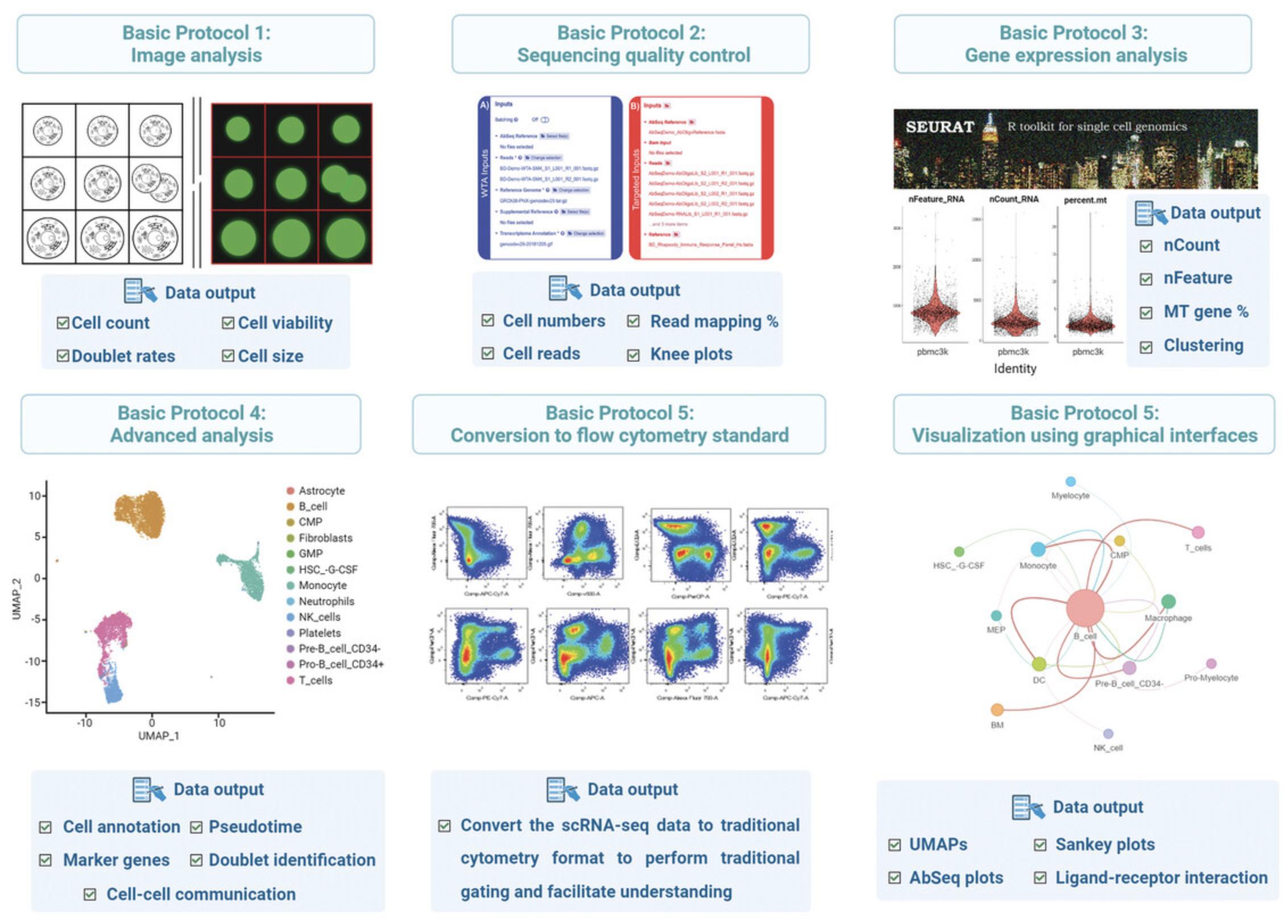
The methods are predominantly implemented in R, and our protocols allow biologists or investigators with minimal informatic experience the ability to process the data.

STRATEGIC PLANNING

Before initiating the analysis and using the proposed workflow for single-cell multiomic data analysis with the BD Rhapsody platform, we recommend that the investigator performs QC checks on the data produced during the wet lab component. Each individual investigator must have their own strategic plans and pay careful attention to the data generated during the experiments. Experimental considerations have been covered by others (Nguyen et al., 2018); however, the specific criteria against which these QC measures are assessed is experiment specific, and the following should be considered:

1. What is the acceptable viability for your sample? Minimum viability has often been stated to be at >90%; however, some situations require the use of cell populations with poor viabilities (such as ultra-rare primary samples or samples in which cell death is being studied). Having low cell viability may be acceptable, but it should be noted and considered during analysis, as it will create data with higher background noise.
1. How many cells were loaded onto the cartridge? There are no rules for the minimum number of cells to be loaded; in theory, even only one cell may get captured. However, only one single cell is unlikely to tell you much about the sample, and as a general rule in scRNA-seq, we try to capture more than 20 cells for our smallest anticipated cell cluster (Luecken & Theis, 2019).
1. How many doublets are you expecting? The upper limit of cartridge loading is restricted by the number of doublets you are willing to accept. Although informatics approaches can be used to infer putative doublets (the anticipated doublet rate is provided in Fig. 2) and sample multiplexing can be used to identify samples of different origins, these systems are not perfect. Therefore, not all doublets can be removed. If remnant doublets are likely to confound your analysis, you should strive to load a total cell number that gives a very low doublet rate.
1. Did the libraries meet the specification in terms of yield and fragment size? Acceptable metrics at each stage are provided in the BD Rhapsody library preparation user guide available on the BD Biosciences Scientific Resources website.

The basic protocols provided in this article have been designed to be used by biologists with a basic knowledge of R; however, we still highly recommend engaging a bioinformatician at the beginning of the experimental planning process. The tools provided are a mechanism by which a user can explore their data and allow for meaningful engagement alongside the advice of an expert bioinformatician.

Considerations before Initiating the Data Analysis

Our basic protocols are built upon R, a programming environment and language utilized for data analytics. For investigators to follow the current set of protocols and generate the same data analysis, before doing the analysis, we recommend the following:

1. Download and install all relevant software (The following example set of software is compatible with Windows systems. Corresponding software for MacOS is also available.) The following are the necessary files to be downloaded:
- R; the version used is R-4.2.1-win.exe. R is a free and open-source programming language. Link to download: https://cran.r-project.org/bin/windows/base/old/4.2.1
- R Studio; the version used is RStudio-2022.07.2-576.exe. RStudio is an Integrated Development Environment (IDE) assisting in program development within R and allowing users to interact with R more readily. Link to download: https://docs.posit.co/previous-versions/rstudio/
- RTools; the version used is rtools42-5355-5357.exe. RTools is a set of programs required to build R packages from source. Link to download: https://cran.r-project.org/bin/windows/Rtools/rtools42/rtools.html
1. Install the required R libraries. First, the tools for package installations must be installed, and then, the required library packages must be downloaded. These packages can be downloaded from a variety of sources; however, the most popular ones are CRAN, Bioconductor, and GitHub.
a) Install tools for package installation. A window may pop up with a question, asking “Do you want to install from source the package which needs compilation” Click “Yes” to continue. The installation of these packages may take a longer time than the other packages. The tools are as follows:
- install.packages('BiocManager')
- install.packages('remotes')
- install.packages('devtools')
b) Make sure to install all required libraries before initiating the basic protocols. A separate script has been provided with this article, called “Current Protocol Packages installation,” to install all the libraries required for this tutorial. The packages used in this article are shown in Table 1.
1. Download the analysis scripts used in this article:
- Current Protocol Packages installation.Rmd
- Current Protocol Basic Protocol 1.Rmd
- Current Protocol Basic Protocol 3.Rmd
- Current Protocol Basic Protocol 4.Rmd
- Current Protocol Basic Protocol 5.Rmd
- Current Protocol Basic Protocol 6.Rmd
- Current Protocol Supplementary mouse.Rmd
- Protocol Supp CellphoneDB.Rmd
- Cell-cell communication analysis with CellphoneDB.docx
1. For those interested in replicating the data generated in the study described here prior to analyzing their own data, the raw data on which the analysis has been carried out are provided in the Supporting Information. We recommend that investigators download and save the data on their computer in a user-specified location. The data files discussed in Table 2 have been provided in the Supporting Information. We encourage the user to download the files individually, unzip them (if necessary), and place them within a folder that they plan to use as their working directory (see next step).
1. Create the working directory and set up the structure so it is compatible with the provided scripts.
a) Users of RStudio software can either create a New Directory from the New Project within the File menu of the RStudio software or make their existing folder in their computer as the working directory via the “Set as Working Directory” function of the RStudio software.
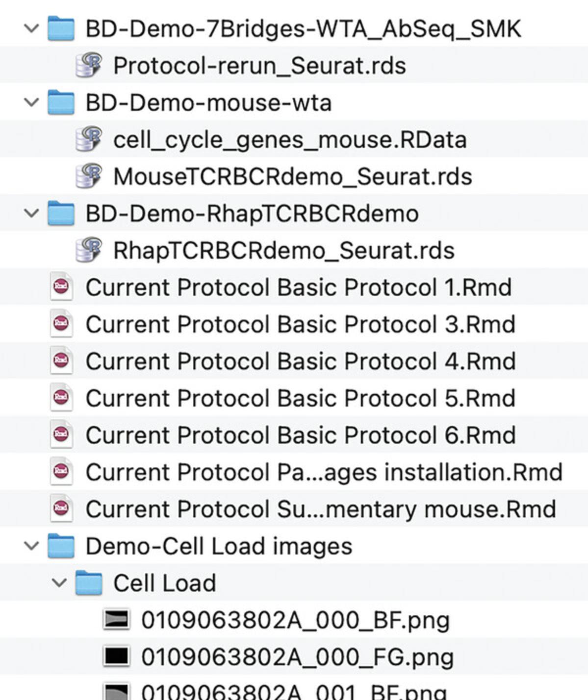
b) Ensure that the folder structure is as shown in Figure 4. If you only want to perform human-related data analysis, there is no need for the “BD-Demo-mouse-wta-abseq” folder.

Table 1. R Packages Used for Data Analysis in the Protocols

Package name	Version	Used in	Source	Reference
magick	2.7.3	Basic Protocol 1	CRAN	(Ooms, 2022)
tidyverse	1.3.2	Basic Protocols 1, 3, 6	CRAN	(Wickham et al., 2019)
ggplot2	3.4.0	Basic Protocols 1, 3, 4	CRAN	(Wickham & SpringerLink, 2009)
Seurat	4.3	Basic Protocols 1, 4, 5, 6	CRAN	(Hao et al., 2021)
harmony	0.1.1	Basic Protocol 4	CRAN	(Korsunsky et al., 2019)
patchwork	1.1.2	Basic Protocols 3, 4	CRAN	(Pedersen, 2020)
rstudioapi	0.14	Basic Protocols 1, 3, 4	CRAN
colorRamps	2.3.1	Basic Protocol 4	CRAN
viridis	0.6.2	Basic Protocol 4	CRAN	(Scherer, 2021)
ape	5.7-1	Basic Protocol 3	CRAN	(Paradis et al., 2019)
EBImage	4.40.0	Basic Protocol 1	Bioconductor	(Pau et al., 2010)
celldex	1.8.0	Basic Protocol 4	Bioconductor	(Aran et al., 2019)
SingleR	2.0.0	Basic Protocol 4	Bioconductor	(Aran et al., 2019)
slingshot	2.6.0	Basic Protocol 4	Bioconductor	(Street et al., 2018)
ComplexHeatmap	2.18.0	Basic Protocol 4	Bioconductor	(Gu et al., 2016)
InterCellar	2.4.0	Basic Protocol 6	Bioconductor	(Interlandi et al., 2022)
romanhaa/cerebroApp	1.3.1	Basic Protocol 6	Bioconductor	(Hillje et al., 2020)
flowCore	2.10.0	Basic Protocol 5	Bioconductor	(Hahne et al., 2009)
chris-mcginnis-ucsf/DoubletFinder	2.0.3	Basic Protocol 4	GitHub	(McGinnis et al., 2019)
satijalab/seurat-wrappers	0.3.1	Basic Protocol 4	GitHub	(Rahul Satija et al., 2020)
cole-trapnell-lab/monocle3	1.3.1	Basic Protocol 4	GitHub	(Cao et al., 2019; Qiu et al., 2017; Qiu et al., 2017; Trapnell et al., 2014)
sqjin/CellChat	1.6.1	Basic Protocol 4	GitHub	(Jin et al., 2021)
immunogenomics/presto	1.0.0	Basic Protocol 4	GitHub	(Ilya Korsunsky et al., 2022)

Table 2. Data Provided for Use in the Protocols

Folder	Description	Used in	Notes
Demo-Cell Load images	For the sake of this study, we have provided our own data for the analysis	Basic Protocol 1	Experimental results output from the BD Rhapsody™ Scanner. The folder contents containing the images are obtained during the “Cell Load” step, and the .csv files contain the coordinates of each cell in the images.
BD-Demo-7Bridges-WTA_AbSeq_SMK	WTA+AbSeq generated from 10,000 resting human PBMCs. Contains six .csv files and one .st matrix.	Basic Protocols 3, 4, 5, and 6. This is referred to as demo exp 1.	Available through BD Biosciences online resources
BD-Demo-RhapTCRBCRdemo	WTA+AbSeq+TCR/BCR from resting human PBMCs and enriched human B cells. Contains eight .csv files, 3 gzip compressed archive files, and 2 ZIP files.	Basic Protocols 3, 4, 5, and 6. This is referred to as demo exp 2.	Available through BD Biosciences online resources
BD-Demo-mouse-wta-abseq	Splenocytes were isolated from the mouse and then stained with a 13plex AbSeq panel, followed by a WTA pipeline. Needs to be independently downloaded.	Supporting Information (Current-Protocol-Supplementary-Mouse	The folder contents are not freely available on the BD Biosciences website and have been provided by the BD Biosciences team

Folder structure of the working directory required for the protocols to function without modification. The working directory contains four folders: three of them hold the gene expression matrices and corresponding sample tag calls if available, and the other one contains the images and .csv files obtained from the BD Rhapsody™ Scanner. If creating your own script, it must be saved within the working directory.

Basic Protocol 1: IMAGE ANALYSIS

The BD Rhapsody™ Single-Cell Analysis System consists of two main platforms, the BD Rhapsody™ Scanner and BD Rhapsody™ Express. The scanner is an automated microscope equipped with a low-magnification objective that produces batches of images at each single-cell capture step. For a complete cycle of single-cell capture, the image output folders are “Cell Load,” “Bead Load,” “Beads Wash,” and “Retrieval.” Each folder contains 26 pairs of bright-field and fluorescence images, except for “Bead Load,” and all folders have a subfolder called “IA_Result.” This folder contains 26 .csv files recording fluorescence information and can be used to locate cells with detectable fluorescence levels.

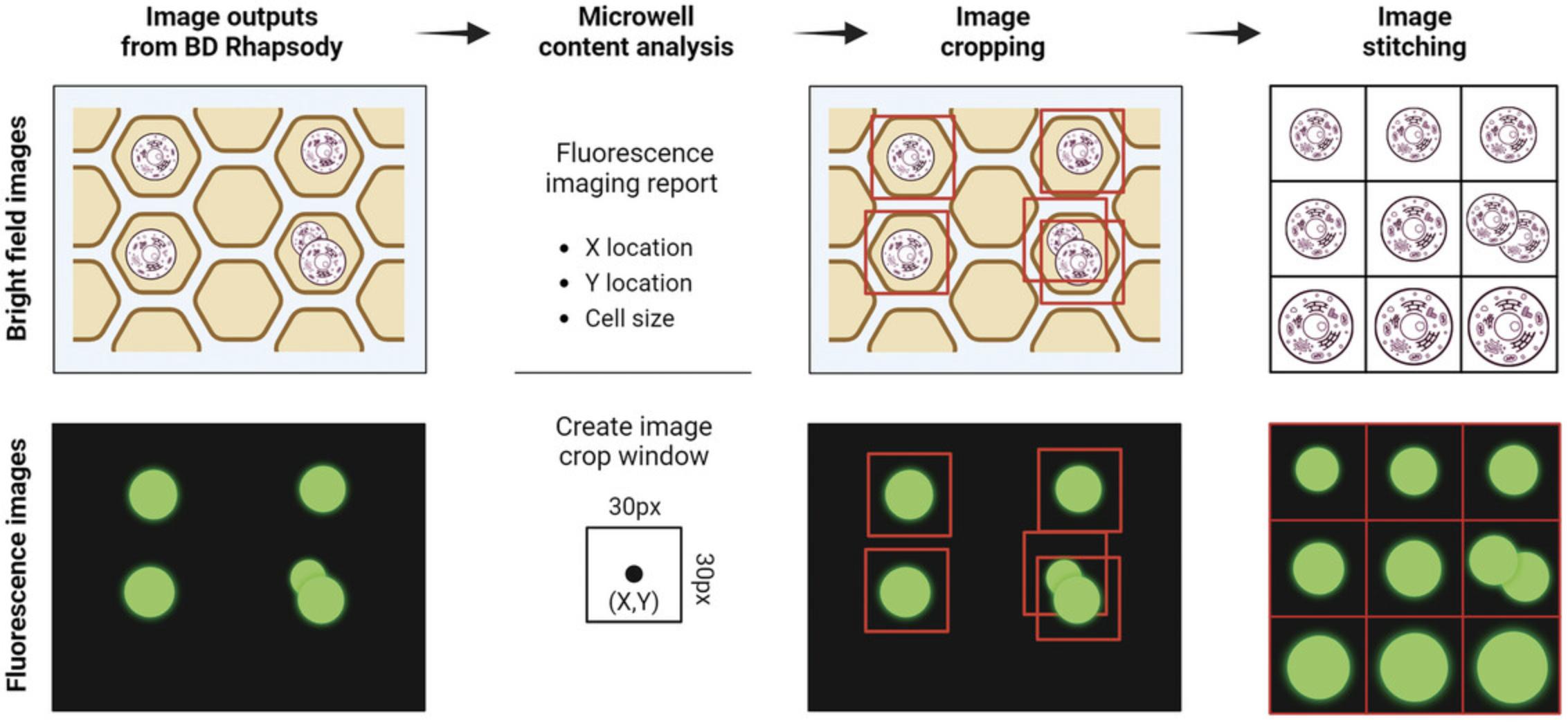
This protocol is constructed in such a way as to take advantage of information contained in the .csv files to pull out image regions that contain putative cell content automatically. Cropped image regions can be ranked by cell size, which is defined by the corresponding fluorescence signal. The workflow is illustrated in Figure 5.If not using the data provided, it is possible to copy the “Cell Load” folder from the BD Rhapsody™ Scanner into the “Demo-Cell Load images” folder within the working directory folder.

Overview of Basic Protocol 1. The workflow has three major steps: (1) collect the location and size information for each cell; (2) loop through each image and crop out wells that contain at least one cell; and (3) stitch cropped images as one image or stack images in .gif format.

Relevance

The ability to image cells that have been captured in high-throughput scRNA-seq systems is unique to the BD Rhapsody. Imaging cells immediately prior to capture for scRNA-seq is important, as it allows accurate determination of doublet rates for every sample, allows quantitation of cell viability (through Calcein AM positivity and DRAQ7 negativity), provides visualization of basic cell properties such as size, and allows visualization of potential clusters.

Current Limitations

The imaging quality is suitable for cell counting and basic size-based statistics. It is unlikely to be suitable for more advanced analysis, such as label-free analysis.

Anticipated Results

Following this image analysis protocol, you will have outputted image files saved on your local computer. These images allow visualization of the cells found in the cartridge during the cell load scan. The processed images possess the same resolution as the input images, except when images are presented in the form of .gif, as these have been digitally magnified 3×. Figure 6 shows an example of images produced using the default cut-offs (0-8 μm, 8-11 μm, and >11 μm) provided in the script. Should user-defined size ranges be required, they should be entered into the script during parameter setting in step 3 using the cell_size_cutpoint command.

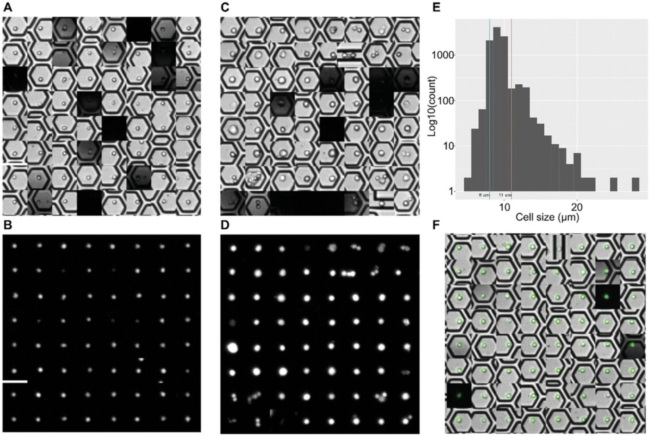
Representative images produced from Basic Protocol 1 for cells of sizes ranging from 8 to 11 μm and >11 μm, respectively. (A) and (B) Representative array of 64 cells with sizes of 8 to 11 μm imaged by brightfield and fluorescence, respectively. (C) and (D) Representative array of 64 cells with sizes of >11 μm imaged by brightfield and fluorescence, respectively. (E) Histogram of the cell size distribution for all cells. (F) Overlay image of bright-field and fluorescence images for 64 cells.

Separating the images of cells above a certain size threshold helps in locating large cells and multiplets and provides a unique glimpse into sample heterogeneity. In the context of circulating tumor cells obtained from the blood, it creates another layer of data, supporting the determination of tumor cells, which tend to be larger than other cells. This feature, not supported by other current high-throughput scRNA-seq platforms, is unique to BD Rhapsody system, and a significant utility is the QC of primary samples.

Necessary Resources

Software access : RStudio (≥2022.07.2 Build 576), R (≥4.2.1)
R packages :
- library(rstudioapi)
- library(magick)
- library(EBImage)
- library(tidyverse)
- library(ggplot2)
Vignette dataset : Demo-Cell Load images are provided in the Supporting Information. If using data from other captures, the data can be found in two file locations on any BD Rhapsody™ Scanner, Local Disk (C:)/ProgramData/Cellular-Research/Experiments (BD Rhapsody™ Scanner images) and Local Disk (C:)/Users/Public/Public Documents/Rhapsody Data (.csv files of cell load information). The folder with BD Rhapsody™ Scanner images also contains a series of corresponding .csv files where cell locations spotted in the cartridge are stored.
Data location : These data should be stored in the folder “Demo-Cell Load images,” as outlined in the previous section (Fig. 4).
NOTE : The script is built in a way that requires minimum manual adjustments. We recommend using a 30 × 30–pixel window to crop out each cell and use 3× zoom-in to display images in .gif format. The images can be divided into groups by size, a quick way to visualize potential tumor cells in the sample. The processed images are generated in the final step (step 12), as outlined below.

1.Having created a new folder on the local computer as per instructions in the “Considerations before initiating the data analysis” section of Strategic Planning, double-check to ensure that the “Cell Load” folder is contained within a sub-folder called “Demo-Cell Load images.” From here, tell R that this folder is where all the data can be found.

# load required packages

library(rstudioapi)

# Obtain the path of this rmarkdown file and assign it to object "get_path"

get_path <- dirname(rstudioapi::getSourceEditorContext()$path)

# Set "get_path" as Working Directory

setwd(get_path)

# Assign 'Demo-Cell Load images' folder path to "cur_path_image"

cur_path_image <- paste(dirname(rstudioapi::getSourceEditorContext()$path),

"Demo-Cell Load images",

sep = "/")

2.Load the required libraries.

# load required packages

library(magick)

library(EBImage)

library(tidyverse)

library(ggplot2)

3.Begin setting up the parameters by setting a minimal 30 × 30–pixel area to capture an entire micro-well (variable is crop_size), setting image magnification to 3× for saving .gif images (variable is image_zoom_times), and setting cell size cut-off points to divide the cropped images into groups (variable is cell_size_cutpoint).

Note

Be aware that the cell size here is determined by the detectable fluorescence signals. Hence, the measurements of cell sizes may not always reflect the true sizes. Users can choose the range most suitable for their experiments. In this step, the cells are divided into three groups according to these ranges: [0-8 μm, 8-11 μm, and >11 μm]. Users can adjust these parameters according to their own experiments.

# User define parameters

# These numbers mean [0 to 8um], [8um - 11um] and [11um to Infinity].

# The cells will be divided into 3 groups based on sizes.

cell_size_cutpoint <- c(0, 8, 11, Inf)

# set image crop size to 30px by 30px

crop_size <- c(30, 30)

# set image zoom in to 3x (for GIF output only)

image_zoom_times <- 3

4.Format the input parameters for the functions and R packages.

# format parameters

crop_size_3_times_zoom <- crop_size*image_zoom_times

crop_shift <- floor(crop_size/2)

crop_size <- paste(crop_size,crop_size,sep = "x")

crop_size_3_times_zoom <- paste(crop_size_3_times_zoom,

crop_size_3_times_zoom,

sep = "x")

cell_group_labels <- sapply(cell_size_cutpoint,

FUN = function(y)

ifelse(y != cell_size_cutpoint[length(cell_size_cutpoint)],

paste0(y, "-", cell_size_cutpoint[grep(y,cell_size_cutpoint)+1],

" um"), y))[-length(cell_size_cutpoint)]

folder_name <- strsplit(cur_path_image,split = "/") %>%

unlist() %>%

.[length(.)]

5.Create an output folder to store processed images.

# Create output folder.

ifelse(!dir.exists(file.path(cur_path_image,

"Image Output")),

dir.create(file.path(cur_path_image,

"Image Output")),

FALSE)

6.Select the “Cell Load” folder to analyze.

# Image folder

subfolder_name <- "Cell Load"

7.Gather image information and create place holders for outputs.

# Gather image information

input_info <- list()

input_info[["image.files.path"]] <- paste(cur_path_image,

subfolder_name ,

sep = "/")

input_info[["csv.files.path"]] <- paste(cur_path_image,

subfolder_name,

"IA_Result",

sep = "/")

input_info[["BF.image.files"]] <- list.files(path = input_info[["image.files.path"]],

pattern = "*.BF.png")

input_info[["FG.image.files"]] <- list.files(path = input_info[["image.files.path"]],

pattern = "*.FG.png")

input_info[["csv.files"]] <- list.files(path = input_info[["csv.files.path"]],

pattern = "*.BF.csv") # One set of files

input_info[["file.length"]] <- length(input_info[["csv.files"]])

8.Load the func_image_crop function.

Note

This is created for cropping images of cells with fluorescence and obtaining their corresponding diameters. The cell images, diameters, and locations are stored in separate R objects.

# function to crop images

func_image_crop <- function(file_length,

image_folder_name,

crop_region,

crop_shift_offset,

csv_files_path,

image_files_path,

image_files_list,

csv_files_list){

# create an empty vector to collect output images from the below looping

image.vector = c()

# create an empty object to collect cell sizes

cell.sizes.vector = c()

# create an empty data frame to collect detailed cell information

cell.sizes.centres.dataframe = c()

# A loop to scan every image and csv file

for (i in 1:file_length){

# Load csv summary file. Skip first 49 lines to make sure the matrix has >4 columns

x.csv <- read.csv(paste(csv_files_path ,

csv_files_list[i],

sep = "/"),

skip = 49,

na.strings = "NA",

header = F)

# Locate cell positions

cell.content.row <- match("Cell Diameter(um)",

x.csv[,2])

# x.csv file tidy-up

# subset the 1-4 columns and rows with cell content information

x.csv <- x.csv[grepl("FG#",x.csv[,1]),

1:4]

x.csv <- x.csv[as.numeric(rownames(x.csv)) > cell.content.row,]

# re-name column names

colnames(x.csv) <- c("CellID",

"CellSize",

"X_centre",

"Y_centre")

rownames(x.csv) <- x.csv$CellID

# move CellID to row names

x.csv <- as.data.frame(x.csv[,c("CellSize",

"X_centre",

"Y_centre")])

cell.sizes.centres.dataframe <- rbind(cell.sizes.centres.dataframe,

x.csv)

temp <- as.data.frame(as.numeric(x.csv$CellSize))

# Final output of all cell sizes in a data frame

cell.sizes.vector <- rbind(cell.sizes.vector,

temp)

# load corresponding image

image.load <- image_read(paste(image_files_path,

image_files_list[i],

sep = "/"))

# First dummy image from the loaded image in order to append subsequent cropped images

image.all <- image_crop(image.load,

crop_region)

# Loop to find cells based on x.csv cell content information

for (j in 1:length(x.csv$X_centre)) {

geometry <- paste(crop_region,

as.numeric(x.csv$X_centre[j])-crop_shift_offset,

as.numeric(x.csv$Y_centre[j])-crop_shift_offset,

sep = "+")

image.crop <- image_crop(image.load,

geometry)

image.all <- c(image.all,

image.crop)

} # end of "for" loop to find cells based on x.csv cell content information

# get rid of the first dummy image

image.all <- image.all[-1]

# add all the images into a vector (here called "image.vector")

image.vector <- append(image.vector,

image.all)

} # end of loop to scan every image and csv file

# Return processed data

return(list(images_cropped = image.vector,

cell_sizes_column = cell.sizes.vector,

cell_size_centre_dataframe = cell.sizes.centres.dataframe))

} # end of "func_image_crop" function

9.Load the func_images_combine function.

Note

This function takes the inputs from the func_image_crop, re-orders them based on cell sizes, and stitches them together as one image.

# function to combine images into one (not stacking & not overlaying)

func_images_combine <- function(image_vector){

image.chunks <- split(image_vector,

ceiling(seq_along(image_vector)/floor(sqrt(length(image_vector)))))

image.chunks.stackFalse <- lapply(image.chunks,magick::image_append,

stack = F)

image.whole <- image.chunks.stackFalse[[1]]

for (i in 1:(length(image.chunks.stackFalse)-1)) {

image.whole <- image_append(c(image.whole,

image.chunks.stackFalse[[i+1]]),

stack = T)

} # end of “for” loop

return(image.whole)

} # end of “func_images_combine” function

10.Load the func_image_gifs_and_image_vector_based_on_cell_size.

Note

This divides cell images into groups based on size. The subsetted images are then converted to .gif and a combined image array for each size range chosen.

## function to create GIFs based on size cutoffs and return cell groups by cutoff sizes

func_image_gifs_and_image_vector_based_on_cell_size <- function(

cutpoint = cell_size_cutpoint,

labels = cell_group_labels,

image_vector,

zoom_region,

toCreateGIF,

cell_sizes_vector # output from function func_image_crop

){

index_temp <- 1:length(image_vector)

cell_sizes <- cell_sizes_vector$`as.numeric(x.csv$CellSize)`

temp.cut <- cut(cell_sizes,

cutpoint,

labels)

temp <- table(temp.cut)

temp.labels <- names(temp[temp !=0])

temp.image.vector.list <- as.list(temp.labels)

names(temp.image.vector.list) <- temp.labels

temp.image.vector.list <- lapply(temp.image.vector.list,

FUN = function(x)

image_vector[index_temp[temp.cut == x]])

temp.image.gif.list <- list()

# Create gifs

if (toCreateGIF) {

for (i in names(temp.image.vector.list)) {

temp.image.gif.list[[i]] <- image_animate(image_scale(temp.image.vector.list[[i]],

geometry = zoom_region),

fps = 4,

dispose = “previous”)

} # end of “for” loop

} # end of “if” statement to create gifs

# Return processed data

return(list(image.vector = temp.image.vector.list,

image.gif = temp.image.gif.list))

} # end of func_image_gifs_and_image_vector_based_on_cell_size function

11.Load the func_batch_output function.

Note

This is used to wrap all the image processing protocols into one automated function. In addition to automating the image analysis protocol, the func_batch_output function has additional features that include artificially colorizing grayscale images, overlaying fluorescence images and brightfield images, creating a cell size distribution histogram, and exporting processed images to the local drive (users can run each function individually with appropriate inputs; however, results will not be saved).

# function to generate image overlays and save final processed images

func_batch_output <- function(

file.length,

subfolder,

crop_size,

crop_shift,

csv.files.path,

image.files.path,

BF.image.files,

FG.image.files,

csv.files,

crop_size_3_times_zoom,

makeGIF,

save_image

){

# Starting time

start_t <- Sys.time()

# call func_image_crop function to process bright field images

image.crop.all.BF <- func_image_crop(file_length = file.length,

image_folder_name = subfolder,

crop_region = crop_size,

crop_shift_offset = crop_shift,

csv_files_path = csv.files.path,

image_files_path = image.files.path,

image_files_list = BF.image.files,

csv_files_list = csv.files)

# call func_image_crop function to process fluorescence images

image.crop.all.FG <- func_image_crop(file_length = file.length,

image_folder_name = subfolder,

crop_region = crop_size,

crop_shift_offset = crop_shift,

csv_files_path = csv.files.path,

image_files_path = image.files.path,

image_files_list = FG.image.files,

csv_files_list = csv.files)

# Order bright field images based on cell sizes

BF.order <- order(image.crop.all.BF$cell_sizes_column$`as.numeric(x.csv$CellSize)`)

# Combine bright field images into one image

image.combine.BF <- func_images_combine(image.crop.all.BF$images_cropped[BF.order])

# Order fluorescence images based on cell sizes

FG.order <- order(image.crop.all.FG$cell_sizes_column$`as.numeric(x.csv$CellSize)`)

# Combine fluorescence images into one image

image.combine.FG <- func_images_combine(image.crop.all.FG$images_cropped[FG.order])

# Change fluorescence images from white-grey scale to white-green scale

FG.image.combine.trans <- image.combine.FG %>%

as_EBImage(.) %>%

EBImage::channel(.,”asgreen”) %>%

magick::image_read(.)

# call func_image_gifs_and_image_vector_based_on_cell_size to make gifimages

BF.gif.and.image.selection <- func_image_gifs_and_image_vector_based_on_cell_size(

image_vector = image.crop.all.BF$images_cropped,

zoom_region = crop_size_3_times_zoom,

toCreateGIF = makeGIF,

cell_sizes_vector = image.crop.all.BF$cell_sizes_column)

# call func_image_gifs_and_image_vector_based_on_cell_size to make gif images

FG.gif.and.image.selection <- func_image_gifs_and_image_vector_based_on_cell_size(

image_vector = image.crop.all.FG$images_cropped,

zoom_region = crop_size_3_times_zoom,

toCreateGIF = makeGIF,

cell_sizes_vector = image.crop.all.FG$cell_sizes_column)

# combine images from gif as one big image

BF.select.combine <- lapply(BF.gif.and.image.selection$image.vector,

func_images_combine)

# combine images from gif as one big image

FG.select.combine <- lapply(FG.gif.and.image.selection$image.vector,

func_images_combine)

# create overlay image of bright field and fluorescence

BF.FG.merge.all <- image_composite(image.combine.BF,

FG.image.combine.trans,

operator = “blend”)

# Display cell sizes histogram

temp <- image.crop.all.BF$cell_sizes_column

colnames(temp) <- “CellSize”

temp.df <- data.frame(Ref = paste(c(cell_size_cutpoint[-c(1,length(cell_size_cutpoint))]),

“um”),

vals = c(cell_size_cutpoint[-c(1,length(cell_size_cutpoint))]),

stringsAsFactors = FALSE)

cell.size.hist <- ggplot(data = temp,

aes(x = CellSize)) +

geom_histogram(binwidth = 1) +

geom_vline(data = temp.df,

mapping = aes(xintercept = vals,

colour = Ref),

show.legend = F) +

geom_text(data = temp.df,

mapping = aes(x = vals,

y = 0,

label = Ref,

hjust = 1,

vjust = -1)) +

scale_y_log10() +

xlab(“Cell Size (μm)”) +

ylab(“Log10(count)”) +

theme(axis.text = element_text(size = 12)) +

theme(axis.title = element_text(size = 12)) +

theme(plot.title = element_text(size = 14)) +

ggtitle(paste(“Histogram of sample --“,

folder_name))

# Save images option

if (save_image == TRUE) {

image_write(image.combine.BF,

path = paste(cur_path_image,

“Image Output”,

paste0(subfolder,

“ -- “,

“all BF.png”),

sep = “/”))

image_write(image.combine.FG,

path = paste(cur_path_image,”Image Output”,

paste0(subfolder,

“ -- “,

“all FG.png”),

sep = “/”))

image_write(FG.image.combine.trans,

path = paste(cur_path_image, “Image Output”,

paste0(subfolder,

“ -- “,

“all FG (green).png”),

sep = “/”))

image_write(BF.FG.merge.all,

path = paste(cur_path_image,”Image Output”,

paste0(subfolder,

“ -- “,

“all BF-FG overlay.png”),

sep = “/”))

for (i in seq_along(BF.select.combine)) {

image_write(BF.select.combine[[i]],

path = paste(cur_path_image, “Image Output”,

paste0(subfolder,

“ -- “,

names(BF.select.combine)[i],

“ BF.png”),

sep = “/”))

} # end of “for” loop

for (i in seq_along(BF.gif.and.image.selection$image.gif)) {

image_write(BF.gif.and.image.selection$image.gif[[i]],

path = paste(cur_path_image,”Image Output”,

paste0(subfolder,

“ -- “,

names(BF.gif.and.image.selection$image.gif)[i],

“ BF.gif”),

sep = “/”))

} # end of “for” loop

for (i in seq_along(FG.select.combine)) {

image_write(FG.select.combine[[i]],

path = paste(cur_path_image,

“Image Output”,

paste0(subfolder,

“ -- “,

names(FG.select.combine)[i],

“ FG.png”),

sep = “/”))

} # end of “for” loop

for (i in seq_along(FG.gif.and.image.selection$image.gif)) {

image_write(FG.gif.and.image.selection$image.gif[[i]],

path = paste(cur_path_image,

“Image Output”,

paste0(subfolder,

“ -- “,

names(FG.gif.and.image.selection$image.gif)[i],

“ FG.gif”),

sep = “/”))

} # end of “for” loop

ggsave(filename = paste0(subfolder,

“ -- “,

“Cell Size Distribution.png”),

plot = cell.size.hist,

path = paste(cur_path_image,

“Image Output”,

sep = “/”),

dpi = 300)

} # end of if “Save images option” statement

# Return end of run message

# Ending time

end_t <- Sys.time()

print(“Function run time:”)

print(end_t -- start_t)

return(“images saved”)

} # end of “func_batch_output” function

12.Run the automated function that saves image results.

Note

Our tests showed that the function magick::image_animate runs faster in MacOS (M1 chip) than in Windows OS. If the process takes too long, change “makeGIF = TRUE” to “makeGIF = FALSE.” This will speed things up, but the .gif file will not be generated.

# Execute script

cell_load_folder_results <- func_batch_output(

file.length = input_info[["file.length"]],

subfolder = subfolder_name,

crop_size = crop_size,

crop_shift = crop_shift,

csv.files.path = input_info[["csv.files.path"]],

image.files.path = input_info[["image.files.path"]],

BF.image.files = input_info[["BF.image.files"]],

FG.image.files = input_info[["FG.image.files"]],

csv.files = input_info[["csv.files"]],

crop_size_3_times_zoom = crop_size_3_times_zoom,

makeGIF = TRUE, # change TRUE to FALSE to disable gif output

save_image = TRUE

)

Basic Protocol 2: SEQUENCING QUALITY CONTROL AND GENERATION OF A GENE EXPRESSION MATRIX

Next-generation sequencing generates raw data files of fluorescent images in BCL format, which are then converted to FASTQ files during the demultiplexing process. These FASTQ files are then aligned to the appropriate genome reference (i.e., GRCh38 for human samples or GRCm38 for mouse samples), QC is performed to ensure high-quality sequencing reads and alignment, and then gene expression is quantified, which is summarized into a gene expression matrix. For the BD Rhapsody system, the current pipeline to do this is carried out via the SevenBridges Platform (www.sevenbridges.com). SevenBridges is a cloud-computing platform that provides the computing power to process data produced by the BD Rhapsody scRNA-seq workflows.

Relevance

FASTQ files must be aligned to the appropriate genome reference to quantify the gene abundance within each cell and perform downstream analysis. In addition, QC is required at multiple stages throughout the data analysis process, importantly to check metrics of sequencing and alignment quality. Performing QC post-sequencing and alignment is imperative to identify the data quality prior to downstream analysis. If the data are suboptimal, they should be discarded, and depending on the cause of concern, the capture, library preparation, or sequencing should be repeated.

Current Limitations

The version of SevenBridges provided by BD allows users a relatively simple interface in which gene expression matrices can be created using FASTQ files generated from BD Rhapsody libraries. The pipelines can be edited, but care should be taken, as they are complex and involve numerous dependencies for which the introduced alterations can compromise the outcome.

Necessary Resources

Software access : SevenBridges account via the internet
R packages : N/A
Support files :
- WTA scRNA-seq requires a reference genome and a transcriptome annotation file. These files can be downloaded via http://bd-rhapsody-public.s3-website-us-east-1.amazonaws.com/Rhapsody-WTA/. Choose the files that match the pipeline version, i.e., version1.x or version2.x. In this protocol, version2.x is used.
- Targeted scRNA-seq requires a list of gene amplicons in FASTA format corresponding to the panel used. The FASTA files for pre-designed panels already exist in SevenBridges. However, if a custom panel is used, a new FASTA file should be created through BD Biosciences.
- AbSeq panels will also require a FASTA file corresponding to the antibodies used in the panel. This FASTA file can be generated via this web-based tool: http://abseq-ref-gen.genomics.bd.com/.
Vignette dataset : Demo project shared by BD Biosciences
User manuals provided by BD Biosciences : Download BD Single-Cell Multiomics Bioinformatics Handbook and Setup User Guide via https://scomix.bd.com/hc/en-us/articles/360019763251-Bioinformatics-Guides

Data loading and FASTQ processing to create a gene expression matrix

SevenBridges provides access to high-performance computing (HPC) through a web interface that can be accessed for BD Rhapsody data through a login provided by BD Biosciences. To convert a FASTQ file to a gene expression matrix, the following broad processes must occur:

1)FASTQ alignment to the appropriate genome reference and/or mapping to the appropriate SMK, AbSeq, or targeted panel.
2)Collapsing of mapped reads to the individual cell label.
3)Selection of cell labels that represent “putative cells.”
4)Provision of reads in a gene expression matrix.

To achieve this, the following steps should be taken within SevenBridges:

1.Log in to SevenBridges : BD Biosciences will provide Rhapsody users a login to perform the analysis.
2.Create a new project : Select the Projects dropdown and choose “+ Create a project.” Select Memorization (prevents having to redo all analysis if parts of the pipeline fail).
3.Import the relevant application pipelines into the project : Navigate to the APPs tab in the project and add (using the Copy button and then clicking Copy again). Commonly used APPs include the BD Rhapsody™ Sequence Analysis Pipeline and SBG Decompressor CWL1.0.
4.Add data files : Navigate to the Files tab in the project and click “+Add files.” This is usually achieved by uploading from a local source. In the case of large or multiple files, use the FTP/HTTP link provided by your sequencing provider.
5.Unzip and compressed files : If the uploaded data were compressed, unzip the .tar data by navigating to the APPs tab and clicking “Run” on the SBG Decompressor CWL1.0 APP. This is a simple pipeline that can be executed by following the directions provided by the APP.
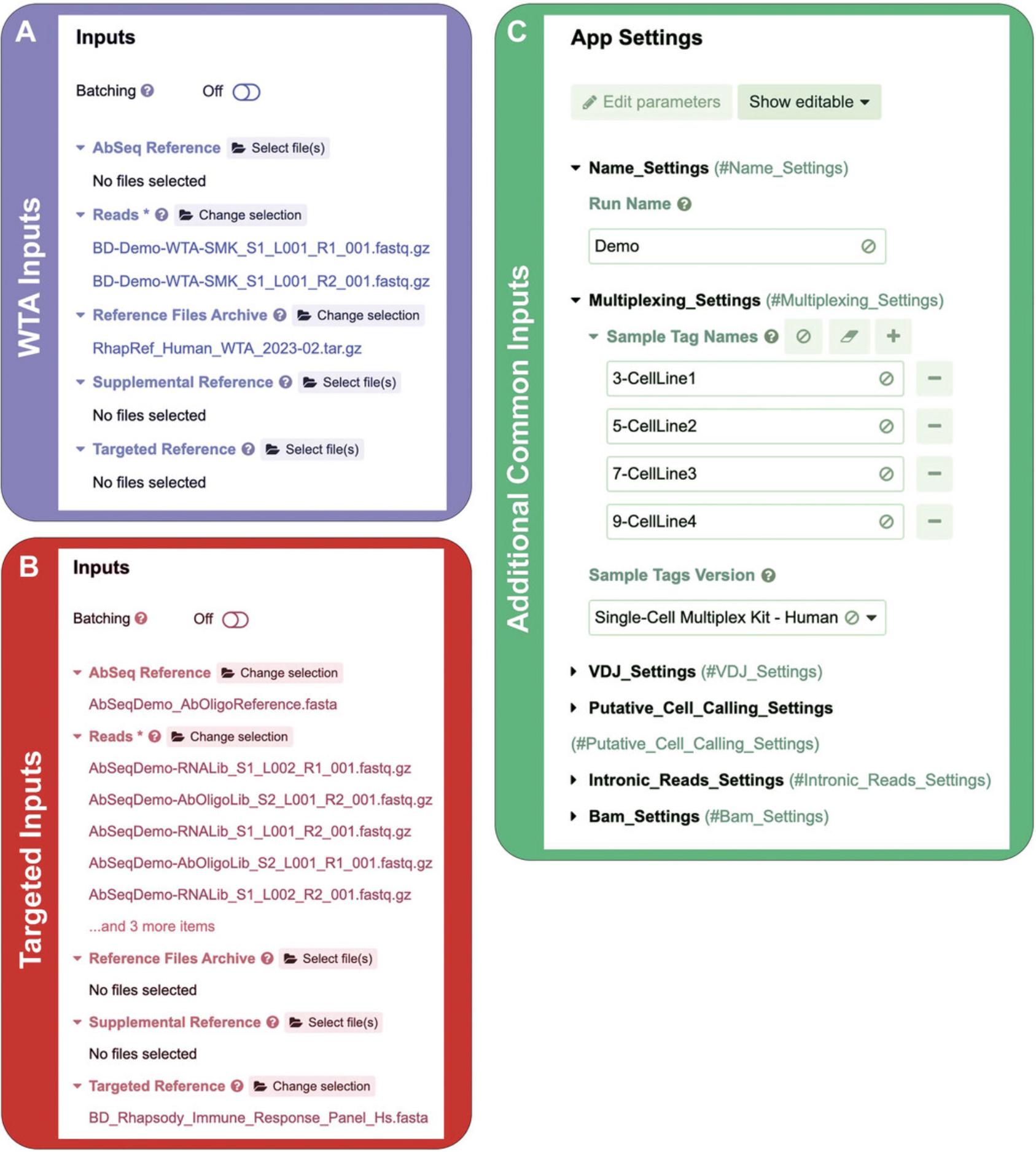
6.Open the BD Rhapsody Pipeline APP : Click run on the BD Rhapsody™ Sequence Analysis Pipeline APP. 0. Check the settings: Provide the input files and ensure the APP settings are correct. Examples of the input files required and the APP setting are shown in Figure7.

Inputs and APP settings required for generating the gene expression matrix from BD Rhapsody data in SevenBridges. (A) Files required for the WTA assay. (B) Files required for the targeted panels. (C) APP settings required. The required fields depend on the assays being run, whether sample tags are used, and if subsampling is required. For more details, please consult the manual provided by BD Biosciences.

7.Execute : Click “Run” to start the pipeline.

Pipeline output from the SevenBridges platform

Upon successful completion of the BD Rhapsody analysis pipeline, the “Output Settings” section will contain these components, including, but not limited to, the BAM file if “Generate Bam Output” was set to “True” in APP settings and the associated index, metrics summary, pipeline report HTML, Scanpy H5AD file, Seurat RDS file and three folders, “Data Tables,” “VDJ” if TCR/BCR profiling was applied, and “Multiplex” if sample tags were applied (Fig. 8).

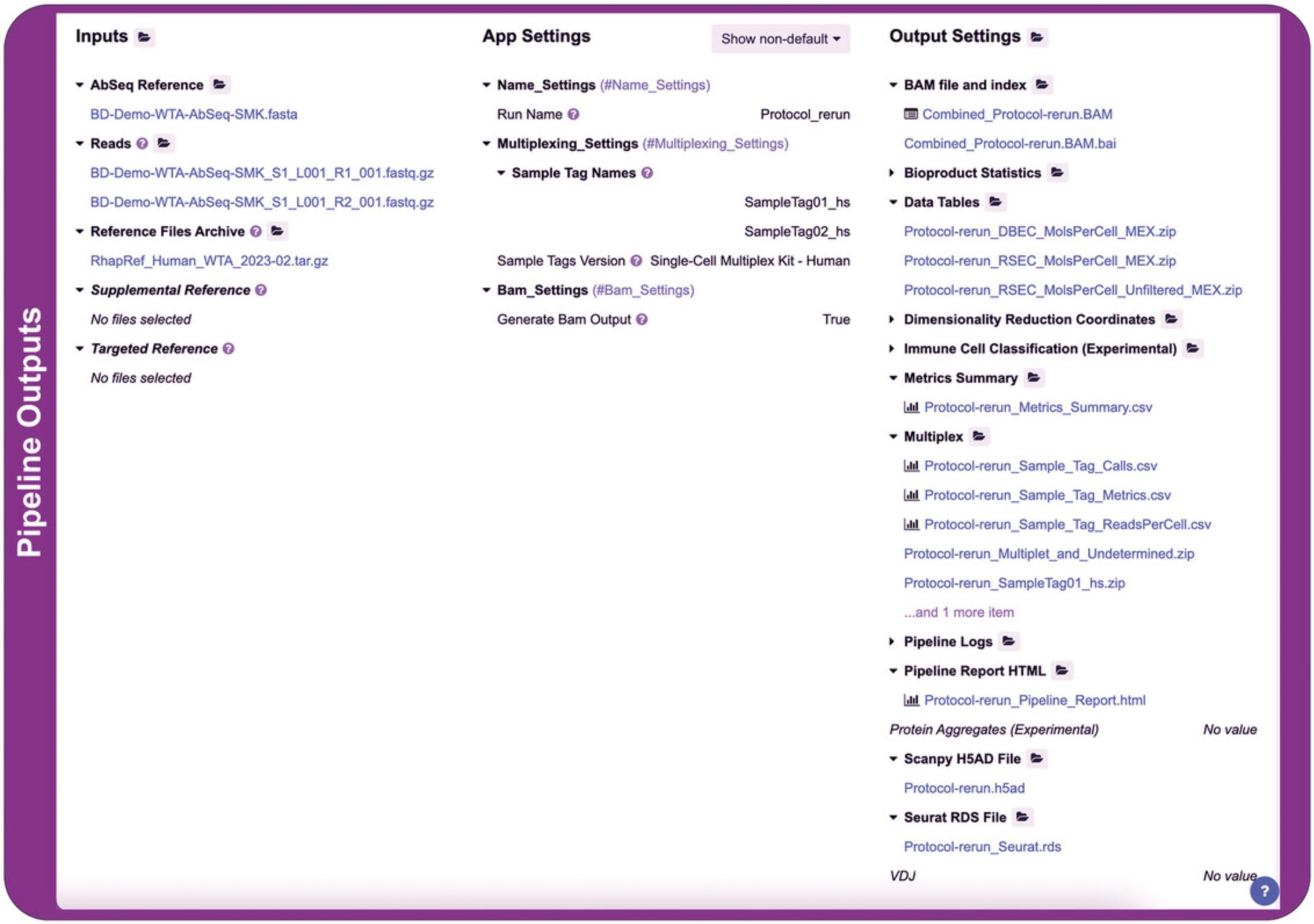
Outputs generated at the end of a successful pipeline run. Files highlighted with red boxes are the inputs for downstream data analysis in subsequent basic protocols utilizing R.

The “Data Tables,” “Seurat RDS file,” and “Scanpy H5AD file” folders can be explained as follows:

1.Data Tables : Two tables (.zip format) will be outputted, respectively containing the number of molecules per cell for all putative cells and all cell labels with at least 10 reads. There are three tsv.gz files in each zipped data table: “barcodes.tsv.gz” for the cell labels, “features.tsv.gz” for the gene list, and “matrix.mtx.gz” for the gene expression matrix.
2.Seurat RDS file and Scanpy H5AD file : The data table with putative cells is converted into a Seurat object and a Scanpy object. If sample tags and/or VDJ profiling were applied, results are included in the metadata of the Seurat object or in the observation data frame of the Scanpy object. The RNA assay of the Seurat object and the data matrix of the Scanpy object contain both an RNA expression matrix and an AbSeq expression matrix if the AbSeq assay was applied.

The BD Rhapsody pipeline on the SevenBridges platform also performs basic QC analysis on the data. Files that provide important information about the QC include the following:

1.Metrics summary : The metrics summary is a .csv file that outlines the statistical overview of an scRNA-seq run through the BD Rhapsody pipeline. It shows the sequencing quality, library quality, percentage of reads aligned, and how many reads per cell.
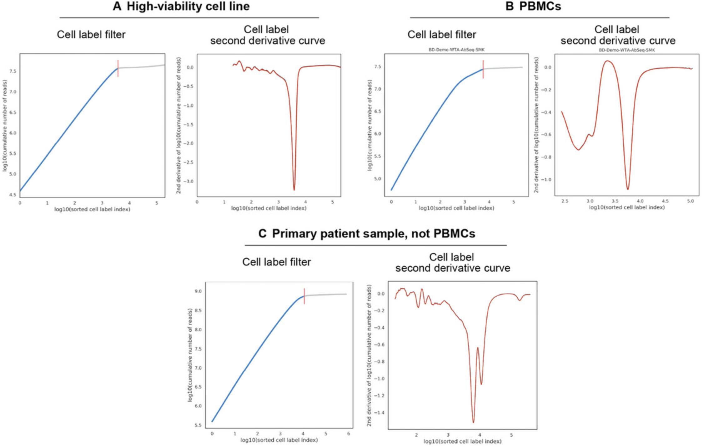
2.Pipeline Report HTML : The report is a stand-alone HTML that contains both the metrics summary of an scRNA-seq run and a section for a cell calling graph. The graph provides a visual representation of the cell quality and the cellular heterogeneity. The blue curve is a graphical indication of the background and reflects the cellular heterogeneity and cell quality, as it shows a plot of the cumulative sequence reads (y -axis) against the number of cell labels identified (x -axis). When the sample is relatively homogeneous, the cumulative curve appears to be linear, and the rate of change in the curve is small. However, as we approach poor-quality cells and the number of reads per cell label decreases, the curve flattens. This turning point is also called the inflection point, indicated by a vertical red line that indicates the numbers of cells the system thinks are present in the data. The same logic can be applied to explain the cumulative curves for heterogeneous samples, which contain populations of cells expressing different levels of genes. Hence, the transition point from one population to another on the cumulative curve can be observed if the difference in mRNA content between the two is large.

The orange curve is an alternate representation that helps to identify the inflection points; these are visualized as rapid drops in the second derivative. Examples with cell calling graphs split into three pairs of plots, the Cell_Label_Filter plots and the Cell_Label_Second_Derivative_Curve plots, for three different sample types are shown in Figure 9. These illustrate the difference between cell lines, namely peripheral blood mononuclear cells (PBMCs) and primary samples (non-PBMCs).

Cell label filter (left) and cell label second derivative curves (right) for different sample input types. Cell lines will often show a very linear cell label plot and a single sharp drop in the second derivative plot (A), whereas samples like PBMCs (B) or primary patient samples (C) may not be so clear.

Basic Protocol 3: GENE EXPRESSION MATRIX DATA PRE-PROCESSING AND ANALYSIS

The Seurat object outputted by the BD Rhapsody SevenBridges pipeline contains a gene expression matrix that links the number of reads for each gene/AbSeq to a specified cell and cell annotations such as cell types, sample tags (if applicable), and TCR/BCR outputs (if applicable). The Seurat object can be loaded to RStudio directly.

This protocol describes how to do the following:

1.Import two example datasets : The first dataset (BD-Demo-7Bridges-WTA_AbSeq_SMK) is a pooled sample with freshly isolated human PBMCs cultured in regular medium for 24 hr (sample tag ID = SampleTag01_hs) and activated PBMCs cultured in the presence of CD3/CD28 for 24 hr (sample tag ID = SampleTag02_hs). The cells were stained with a 20plex AbSeq panel. We use the .rds file from the SevenBridges pipeline, setting this to the “demo_seurat_1” variable in R. The second dataset (BD-Demo-RhapTCRBCRdemo) is a pooled sample with frozen resting human PBMCs (sample tag ID = SampleTag05_hs) and enriched human B cells (sample tag ID = SampleTag06_hs). We use the .rds file from the SevenBridges pipeline, setting this to the “demo_seurat_2” variable in R.
2.Perform normalization, scaling, dimensionality reduction, and clustering on both datasets.
3.Carry out basic visualization for both datasets.

Relevance

Appropriate curation of the Seurat object is necessary for the analysis of an expression matrix that has RNA and protein assays using the R library package Seurat. More detailed information can be found at https://satijalab.org/seurat/articles/get_started.html. An in-depth protocol was previously published (see Current Protocols article: Ji & Sadreyev, 2019), describing how to utilize Seurat to process scRNA-seq data. However, it is based on the Chromium 10× platform. Here, we provide a protocol specific to the output from the BD Rhapsody workflow.

Current Limitations

Seurat provides an alternative way to normalize gene expression data, which is the SCTransform function. This approach handles technical artifacts better; however, it is more time consuming than the method described in this protocol. Therefore, SCTransform is not recommended for large datasets.

Necessary Resources

Software access : RStudio (≥2022.07.2 Build 576), R (≥4.2.1)
R packages :
- library(rstudioapi)
- library(Seurat)
- library(patchwork)
- library(tidyverse)
- library(S4Vectors)
- library(ggplot2)
Vignette dataset : Provided in the Supporting Information:
- Folder name for demo exp 1: BD-Demo-7Bridges-WTA_AbSeq_SMK
- Folder name for demo exp 2: BD-Demo-RhapTCRBCRdemo

1.Set up the environment by loading the relevant libraries and setting the inputs and outputs, and load the function func_save_images to save output images.

# load required packages

library(rstudioapi)

library(Seurat)

library(patchwork)

library(S4Vectors)

library(tidyverse)

library(ggplot2)

# set a seed to re-produce pseudorandom numbers

set.seed(99)

# Obtain the path of this rmarkdown file and assign it to object "get_path"

get_path <- dirname(rstudioapi::getSourceEditorContext()$path)

# Set "get_path" as Working Directory

setwd(get_path)

# Save images and data to this folder

saveTo <- "Protocol 3 output"

# Create a function to save output images

func_save_images <- function(image.object, # plot objects

image.name, # name of the plot

image.path, # path to save image

h = 8, # image height in inch

w = 15, # image width in inch

r = 300, # image resolution

isHeatmap = F # check if image is a Seurat heatmap

){

ifelse(!dir.exists(image.path),

dir.create(image.path,

recursive = T),

FALSE)

if(isHeatmap){

for(i in seq_along(image.name)){

temp.path <- paste(image.path,

image.name[i],

sep = "/")

tiff(filename = paste(temp.path,

"tiff",

sep = "."),

width = w,

height = h,

res = r,

units = "in")

image.object[[i]]

dev.off()

} # end of for 1st loop

}else{

for(i in seq_along(image.name)){

temp.path <- paste(image.path,

image.name[i],

sep = "/")

ggsave(filename = paste(temp.path,

"tiff",

sep = "."),

plot = image.object[[i]],

width = w,

height = h,

units = "in",

dpi = r,

limitsize = FALSE)

} # end of for 2nd loop

} # end of if isHeatmap statement

}# end of func_save_images function

2.Load the two demo Seurat objects and read data.

# Choose a folder/experiment to analyse

exp1 <- "BD-Demo-7Bridges-WTA_AbSeq_SMK"

exp2 <- "BD-Demo-RhapTCRBCRdemo"

# Load the Seurat objects as demo_seurat_1 and demo_seurat_2

demo_seurat_1 <- readRDS(list.files(exp1, full.names = T))

demo_seurat_2 <- readRDS(list.files(exp2, full.names = T))

To check the details and dimensions of the Seurat object created, type the name of the Seurat object into the terminal (shown in code below).

Note

This returns information on the Seurat object created, such as the cell count, features, and assays.

demo_seurat_1

An object of class Seurat

28227 features across 5589 samples within 1 assay

Active assay: RNA (28227 features, 0 variable features)

1 dimensional reduction calculated: tsne

demo_seurat_2

An object of class Seurat

33470 features across 7212 samples within 1 assay

Active assay: RNA (33470 features, 0 variable features)

1 dimensional reduction calculated: tsne

To split the RNA assay into two assays, one for RNA and another for AbSeq, use the following code.

Note

Both of the demo datasets come with an expression matrix from RNA and AbSeq, which is respectively stored in the RNA assay of the Seurat objects.

Note

If your dataset does not contain an AbSeq assay, skip this step.

# Curate the Seurat objects

# get AbSeq list

AbSeq_list_1 <- rownames(demo_seurat_1)[grepl("pAbO", rownames(demo_seurat_1))]

AbSeq_list_2 <- rownames(demo_seurat_2)[grepl("pAbO", rownames(demo_seurat_2))]

# get RNA gene list

RNA_list_1 <- rownames(demo_seurat_1)[!grepl("pAbO", rownames(demo_seurat_1))]

RNA_list_2 <- rownames(demo_seurat_2)[!grepl("pAbO", rownames(demo_seurat_2))]

# subset demo_seurat_1 and demo_seurat_2 by AbSeq and RNA gene lists

demo_AbSeq_1 <- subset(demo_seurat_1,features=AbSeq_list_1)

demo_AbSeq_2 <- subset(demo_seurat_2,features=AbSeq_list_2)

demo_seurat_1 <- subset(demo_seurat_1,features=RNA_list_1)

demo_seurat_2 <- subset(demo_seurat_2,features=RNA_list_2)

# create new Seurat objects

demo_seurat_1@assays[["AB"]] <- GetAssay(demo_AbSeq_1,assay = "RNA")

demo_seurat_2@assays[["AB"]] <- GetAssay(demo_AbSeq_2,assay = "RNA")

# remove demo_AbSeq_1 and demo_AbSeq_2

remove(demo_AbSeq_1, demo_AbSeq_2)

To duplicate the “Sample_Name” cell annotation as “smk” into the metadata, use the following command line.

Note

The sample tagging information of the demo datasets is stored in the metadata of the Seurat object as “Sample_Tag” and “Sample_Name.”

demo_seurat_1$smk <- demo_seurat_1$Sample_Name

demo_seurat_2$smk <- demo_seurat_2$Sample_Name

Type the name of the Seurat object into the terminal again to inspect the updated data structure.

demo_seurat_1

An object of class Seurat

28227 features across 5589 samples within 2 assays

Active assay: RNA (28207 features, 0 variable features)

1 other assay present: AB

1 dimensional reduction calculated: tsne

demo_seurat_2

An object of class Seurat

33470 features across 7212 samples within 2 assays

Active assay: RNA (33430 features, 0 variable features)

1 other assay present: AB

1 dimensional reduction calculated: tsne

3.Perform data normalization, scaling, and clustering.

Note

This step uses func_quick_process to form the basis for all future advanced analyses. Here, we combine the Seurat functions NormalizeData, FindVariableFeatures, ScaleData, RunPCA, RunUMAP, FindNeighbors, FindClusters, PercentageFeatureSet, and BuildClusterTree.

Note

Part of this function involves a QC step, which is needed to negate artifacts such as PCR amplification variations, library preparation inconsistencies, and cell viability. Technical noise generated in the library preparation step is accounted for by normalizing, scaling, and log-transforming the gene expression count matrices. During QC, the proportion of mitochondrial (MT) genes expressed can be checked, as a high percentage of MT genes indicates that the cell has RNA content leakage. The percentage of MT reads that is acceptable can vary with the input; we show how to remove unwanted cells in step 5.

Note

The other aspect of this function is to perform dimensionality reduction. During this step, genes are ranked by the highest degree of variance to the lowest, and by default, the top 2000 genes are used to perform a principal component analysis (PCA). The principal components (PCs) are passed to a dimension reduction algorithm, UMAP, for data visualization and clustering of the cells using their gene expression values.

Note

It is important to note that several normalization methods exist that are different in the degree of complexity. However, differences exist between various normalization methods, and comparing all normalization techniques is still open research to consider. Although some research groups made attempts to compare certain normalization techniques and evaluate their effects on the downstream analysis, these attempts were either incomplete, meaning that the groups did not compare all the existing methods, or resulted in different conclusions (Booeshaghi et al., 2022; Germain et al., 2020; Schneider et al., 2021). For this step-by-step protocol, we have selected the Centered Log Ratio (CLR) method; nevertheless, we encourage the user to evaluate the impact and results of the selected normalization method on the corresponding downstream analysis and select the one that best suits their experiment.

# Build function

# The size of AbSeq panels varies, reduce the number

# for ab_pc_num if your panel is smaller than 10.

func_quick_process <- function(demo_seurat,

ab_pc_num = 10, # number of PCA components to use for protein

rna_pc_num = 15, # number of PCA components to use for RNA

ab_reduction_res = 0.8, # cluster resolution for protein

rna_reduction_res = 0.8) # cluster resolution for RNA

{

# check if the Seurat object has protein assay

if("AB" %in% Seurat::Assays(demo_seurat))

{

Seurat::DefaultAssay(demo_seurat) <- 'AB'

# Normalize and scale data

demo_seurat <- demo_seurat %>%

Seurat::NormalizeData(normalization.method = 'CLR', margin = 2) %>%

Seurat::FindVariableFeatures() %>%

Seurat::ScaleData()

# perform PCA

demo_seurat <- Seurat::RunPCA(object = demo_seurat,

reduction.name = 'apca')

# perform UMAP

demo_seurat <- Seurat::RunUMAP(demo_seurat,

reduction = 'apca',

dims = 1:ab_pc_num,

assay = 'AB',

reduction.name = 'adt.umap',

reduction.key = 'adtUMAP_')

# Find clusters

demo_seurat <- Seurat::FindNeighbors(demo_seurat,

reduction = "apca",

dims = 1:ab_pc_num)

demo_seurat <- Seurat::FindClusters(demo_seurat,

resolution = ab_reduction_res,

graph.name = "AB_snn")

} # end of if statement

# Change default assay to RNA

Seurat::DefaultAssay(demo_seurat) <- "RNA"

# Calculate percentages of mitochondrial gene expression for every cell. If it is a

# targeted sequencing, then the output of this commend line is all zeros.

demo_seurat <- Seurat::PercentageFeatureSet(demo_seurat,

pattern = "^MT[-|.]",

col.name = "percent.mt")

# find top most variant genes

demo_seurat <- demo_seurat %>%

Seurat::NormalizeData() %>%

Seurat::FindVariableFeatures(.,

selection.method = "vst")

# scale data

demo_seurat <- Seurat::ScaleData(demo_seurat,

verbose = FALSE)

# perform PCA

demo_seurat <- Seurat::RunPCA(demo_seurat,

npcs = rna_pc_num,

verbose = FALSE)

# perform UMAP

demo_seurat <- Seurat::RunUMAP(demo_seurat,

reduction = "pca",

dims = 1:rna_pc_num)

# Find clusters

demo_seurat <- Seurat::FindNeighbors(demo_seurat,

reduction = "pca",

dims = 1:rna_pc_num)

demo_seurat <- Seurat::FindClusters(demo_seurat,

resolution = rna_reduction_res)

demo_seurat <- Seurat::BuildClusterTree(demo_seurat)

# return Seurat object as output

return(demo_seurat)

} # end of func_quick_process function

# Use the above function to process the Seurat objects

demo_seurat_1 <- func_quick_process(demo_seurat_1)

demo_seurat_2 <- func_quick_process(demo_seurat_2)

Create a folder to save the Seurat object and save the object to the local drive.

# Create a folder called saveTo

ifelse(!dir.exists(saveTo),

dir.create(saveTo,

recursive = T),

FALSE)

# Save Seurat objects to local drive

save(demo_seurat_1,

demo_seurat_2,

file = paste(saveTo,

"raw demo Seurat objects.RData",

sep = "/")

)

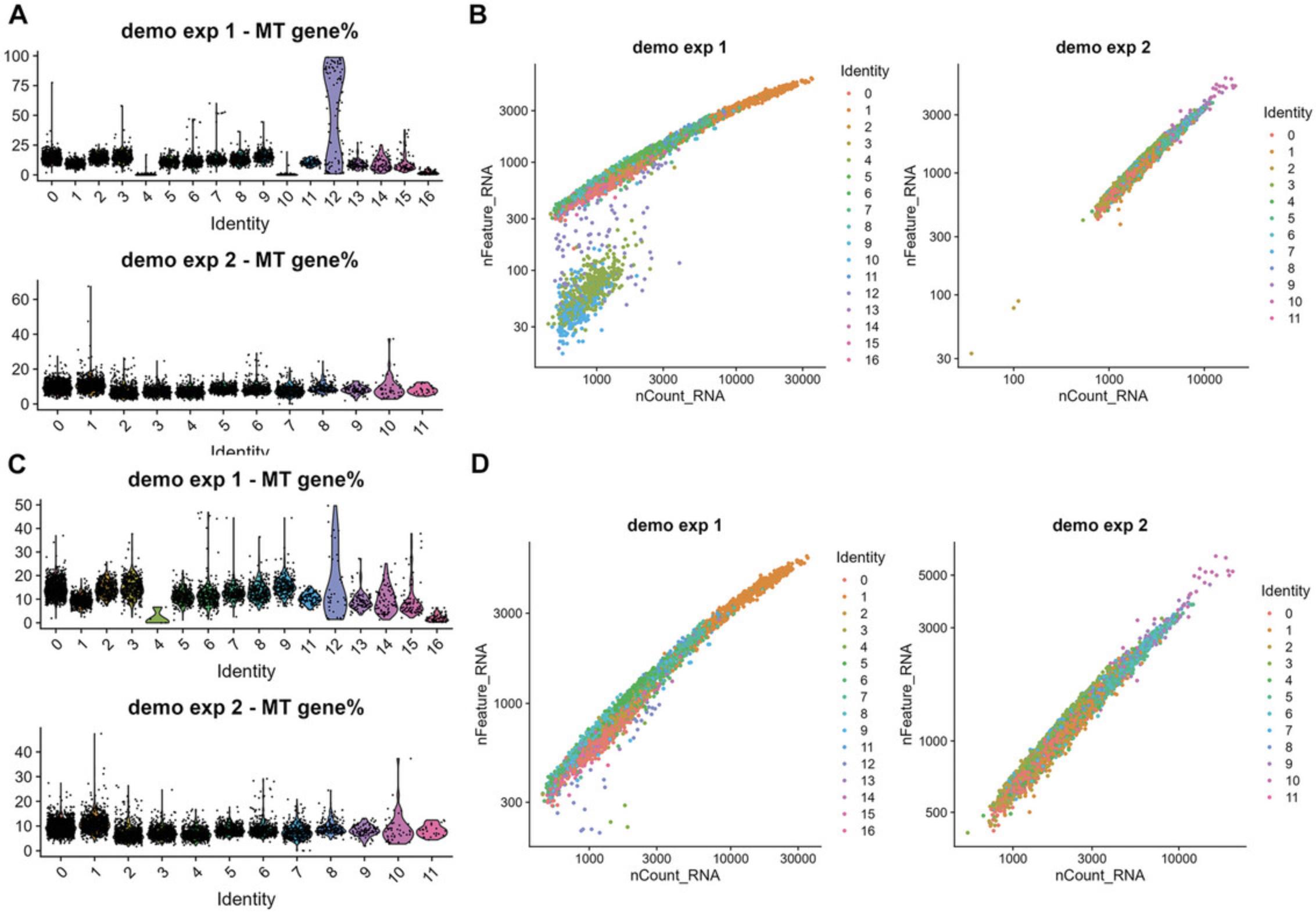
4.Perform removal of poor-quality cells and basic visualization, beginning by producing Violin plots and Feature Scatter plots on all cells in the dataset and saving to a folder using the func_save_images function.

Note

Having performed normalization, scaling, and clustering, we can now visualize the results. There are multiple visualization tools within Seurat. In this step, we use Violin plots (VlnPlot) and Feature Scatter plots (FeatureScatter); both are grouped by the clusters assigned in step 4. The below code generates Figure 10.

# QC plots -- check mitochondrial gene percentages

p1 <- Seurat::VlnPlot(demo_seurat_1,

features = "percent.mt",

group.by = "seurat_clusters") +

Seurat::NoLegend() +

ggtitle("demo exp 1 - MT gene%")

p2 <- Seurat::VlnPlot(demo_seurat_2,

features = "percent.mt",

group.by = "seurat_clusters") +

Seurat::NoLegend() +

ggtitle("demo exp 2 - MT gene%")

patchwork::wrap_plots(p1 + p2)

func_save_images(image.object = list(patchwork::wrap_plots(p1 + p2)),

image.name = "Initial MT genes percentages",

image.path = saveTo,

h = 5,

w = 5,

r = 300,

isHeatmap = F

)

p3 <- Seurat::FeatureScatter(demo_seurat_1,

feature1 = "nCount_RNA",

feature2 = "nFeature_RNA",

group.by = "seurat_clusters") +

scale_x_log10() +

scale_y_log10() +

ggtitle("demo exp 1")

p4 <- Seurat::FeatureScatter(demo_seurat_2,

feature1 = "nCount_RNA",

feature2 = "nFeature_RNA",

group.by = "seurat_clusters") +

scale_x_log10() +

scale_y_log10() +

ggtitle("demo exp 2")

patchwork::wrap_plots(p3 + p4)

func_save_images(image.object = list(patchwork::wrap_plots(p3 + p4)),

image.name = "Initial nCounts and nFeatures",

image.path = saveTo,

h = 5,

w = 11,

r = 300,

isHeatmap = F

)

After visualizing these plots, remove low-quality cells by subsetting high-quality cells into a new Seurat object.

Note

In this case, we chose to subset demo_seurat_1 so that it contains only cells with <50% MT content and with an nFeature_RNA of more than 200. For demo_seurat_2, we subsetted so that the new object contains only cells with <50% MT content and with an nFeature_RNA of more than 100.

# filter out cells with MT genes percentage > 50 (%) and

# cells with low nFeature_RNA

subset_demo_seurat_1 <- subset(demo_seurat_1,

subset = percent.mt < 50 &

nFeature_RNA > 200,

invert = F)

subset_demo_seurat_2 <- subset(demo_seurat_2,

subset = percent.mt < 50 &

nFeature_RNA > 100,

invert = F)

p5 <- Seurat::VlnPlot(subset_demo_seurat_1,

features = "percent.mt",

group.by = "seurat_clusters") +

Seurat::NoLegend() +

ggtitle("demo exp 1 - MT gene%")

p6 <- Seurat::VlnPlot(subset_demo_seurat_2,

features = "percent.mt",

group.by = "seurat_clusters") +

Seurat::NoLegend() +

ggtitle("demo exp 2 - MT gene%")

patchwork::wrap_plots(p5 + p6)

func_save_images(image.object = list(patchwork::wrap_plots(p5 + p6)),

image.name = "Subset - MT genes percentages (before re-clustering)",

image.path = saveTo,

h = 5,

w = 5,

r = 300,

isHeatmap = F

)

p7 <- Seurat::FeatureScatter(subset_demo_seurat_1,

feature1 = "nCount_RNA",

feature2 = "nFeature_RNA",

group.by = "seurat_clusters") +

scale_x_log10() +

scale_y_log10() +

ggtitle("demo exp 1")

p8 <- Seurat::FeatureScatter(subset_demo_seurat_2,

feature1 = "nCount_RNA",

feature2 = "nFeature_RNA",

group.by = "seurat_clusters") +

scale_x_log10() +

scale_y_log10() +

ggtitle("demo exp 2")

patchwork::wrap_plots(p7 + p8)

func_save_images(image.object = list(patchwork::wrap_plots(p7 + p8)),

image.name = "Subset - nCounts and nFeatures (before re-clustering)",

image.path = saveTo,

h = 5,

w = 11,

r = 300,

isHeatmap = F

)

QC visualization plots of the data before and after removing cells with high MT content (>50%) and low gene features (cells with less than 200 and 100 RNA molecules, respectively). (A) and (C) Violin plots showing the MT gene percentage in each cluster before and after removing low-quality cells (demo exp 1 and demo exp 2, respectively). (B) and (D) nCount vs. nFeature plots before and after removing low-quality cells (demo exp 1 and demo exp 2, respectively).

5.Perform dimensionality reduction in high-quality cells.

Note

Having removed low-quality cells, it is important to re-run the func_quick_process. In this step, we are performing normalization, scaling, and dimensionality reduction on the selected high-quality cells from subset_demo_seurat_1 and subset_demo_seurat_2 using the func_quick_process. After this is performed, we can use the DimPlot function in Seurat to visualize the UMAPs for each dataset (Fig. 11).

# Re-cluster subsetted samples

subset_demo_seurat_1 <- func_quick_process(subset_demo_seurat_1)

subset_demo_seurat_2 <- func_quick_process(subset_demo_seurat_2)

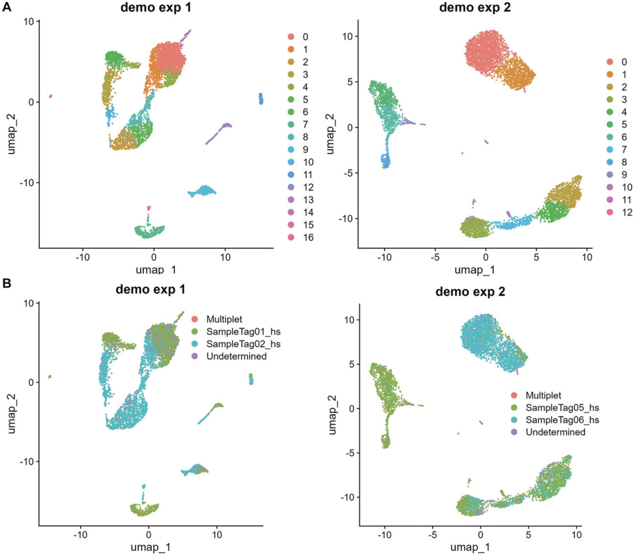
# UMAP plots

p9 <- Seurat::DimPlot(subset_demo_seurat_1,

reduction = "umap",

group.by = "seurat_clusters") +

ggtitle("demo exp 1")

p10 <- Seurat::DimPlot(subset_demo_seurat_2,

reduction = "umap",

group.by = "seurat_clusters") +

ggtitle("demo exp 2")

patchwork::wrap_plots(p9+p10)

func_save_images(image.object = list(patchwork::wrap_plots(p9 + p10)),

image.name = "Subset - UMAP group by clusters",

image.path = saveTo,

h = 5,

w = 11,

r = 300,

isHeatmap = F

)

p11 <- Seurat::DimPlot(subset_demo_seurat_1,

reduction = "umap",

group.by = "smk") +

ggtitle("demo exp 1")

p12 <- Seurat::DimPlot(subset_demo_seurat_2,

reduction = "umap",

group.by = "smk") +

ggtitle("demo exp 2")

patchwork::wrap_plots(p11+p12)

func_save_images(image.object = list(patchwork::wrap_plots(p11 + p12)),

image.name = "Subset - UMAP group by sample tag",

image.path = saveTo,

h = 5,

w = 13,

r = 300,

isHeatmap = F

)

UMAP plots generated in Seurat. Cells highlighted by Seurat cluster ID (A) and cells highlighted by sample tags (B). In both panels, the data for demo exp 1 are provided on the left and for demo exp 2 on the right.

6.Save the high-quality Seurat object.

Note

In this step, the subsetted Seurat objects are saved to the local drive for further advanced analysis introduced in Basic Protocol 4.

# Save Seurat objects to local drive

save(subset_demo_seurat_1,

subset_demo_seurat_2,

file = paste(saveTo,

"subsetted demo Seurat objects.RData",

sep = "/"))

Basic Protocol 4: ADVANCED ANALYSIS

A variety of tools have been developed to support advanced scRNA-seq analysis. It is unrealistic to attempt to introduce all of them in this protocol. Instead, we will demonstrate how to use popular packages to perform the most common advanced scRNA-seq analysis.

This protocol takes the two Seurat objects created in Basic Protocol 3 and performs the following: 1) cell type annotation, 2) merging of datasets and removal of batch effect, 3) finding doublets, 4) finding marker genes, 5) performing pseudotime and trajectory analysis (only shown for subset_demo_seurat_1); and 6) analyzing cell-cell communication.

Relevance

scRNA-seq provides an incredibly rich dataset that can provide a detailed snapshot of the biology of the samples being interrogated at single-cell resolution. Without taking advantage of advanced analysis tools, like those listed here, much of the power of high-throughput single-cell omics will be unexplored.

Current Limitations

There are multiple packages to perform the same type of analysis; however, the tools often return slightly different results. It is beyond the scope of this article to discuss the strengths and weaknesses of each package or the specific use cases for each. We recommend that you consult a bioinformatician to discuss these nuances and use the appropriate package to suit your experimental needs.

Necessary Resources

Software access : RStudio (≥2022.07.2 Build 576), R (≥4.2.1)
R packages :
- library(rstudioapi)
- library(Seurat)
- library(ggplot2)
- library(tidyverse)
- library(patchwork)
- library(celldex)
- library(SingleR)
- library(harmony)
- library(DoubletFinder)
- library(SeuratWrappers)
- library(monocle3)
- library(slingshot)
- library(colorRamps)
- library(CellChat)
Support files : N/A
Vignette dataset : Subsetted demo Seurat objects.RData from Basic Protocol 3

1.Load RData and set up the working environment.

Note

This step loads the required library packages, creates a function to save output images, and loads the subsetted Seurat objects generated in Basic Protocol 3 into the working environment. It also creates a new folder for the results generated.

# load required packages

# load libraries

library(rstudioapi)

library(Seurat)

library(ggplot2)

library(tidyverse)

library(patchwork)

library(celldex)

library(SingleR)

library(harmony)

library(DoubletFinder)

library(SeuratWrappers)

library(monocle3)

library(slingshot)

library(colorRamps)

library(CellChat)

# set a seed to re-produce pseudorandom numbers

set.seed(99)

# Obtain the path of this rmarkdown file and assign it to object "get_path"

get_path <- dirname(rstudioapi::getSourceEditorContext()$path)

# Set "get_path" as Working Directory

setwd(get_path)

# load subsetted Seurat objects for Basic Protocol 3

load("Protocol 3 output/subsetted demo Seurat objects.RData")

# Save images and data to this folder

saveTo <- "Protocol 4 output"

# Create a function to save output images

func_save_images <- function(image.object, # plot objects

image.name, # name of the plot

image.path, # path to save image

h = 8, # image height in inch

w = 15, # image width in inch

r = 300, # image resolution

isHeatmap = F # check if image is a Seurat heatmap

){

ifelse(!dir.exists(image.path),

dir.create(image.path,

recursive = T),

FALSE)

if(isHeatmap){

for(i in seq_along(image.name)){

temp.path <- paste(image.path,image.name[i],

sep = "/")

tiff(filename = paste(temp.path,

"tiff",

sep = "."),

width = w,

height = h,

res = r,

units = "in")

image.object[[i]]

dev.off()

} # end of for 1st loop

}else{

for(i in seq_along(image.name)){

temp.path <- paste(image.path,

image.name[i],

sep = "/")

ggsave(filename = paste(temp.path,

"tiff",

sep = "."),

plot = image.object[[i]],

width = w,

height = h,

units = "in",

dpi = r,

limitsize = FALSE)

} # end of 2nd for loop

} # end of if isHeatmap statement

}# end of func_save_images function

# The size of AbSeq panels varies, reduce the number

# for ab_pc_num if your panel is smaller than 10.

func_quick_process <- function(demo_seurat,

ab_pc_num = 10, # number of PCA components to use for protein

rna_pc_num = 15, # number of PCA components to use for RNA

ab_reduction_res = 0.8, # cluster resolution for protein

rna_reduction_res = 0.8) # cluster resolution for RNA

{

# check if the Seurat object has protein assay

if("AB" %in% Seurat::Assays(demo_seurat))

{

Seurat::DefaultAssay(demo_seurat) <- 'AB'

# Normalize and scale data

demo_seurat <- demo_seurat %>%

Seurat::NormalizeData(normalization.method = 'CLR', margin = 2) %>%

Seurat::FindVariableFeatures() %>%

Seurat::ScaleData()

# perform PCA

demo_seurat <- Seurat::RunPCA(object = demo_seurat,

reduction.name = 'apca')

# perform UMAP

demo_seurat <- Seurat::RunUMAP(demo_seurat,

reduction = 'apca',

dims = 1:ab_pc_num,

assay = 'AB',

reduction.name = 'adt.umap',

reduction.key = 'adtUMAP_')

# Find clusters

demo_seurat <- Seurat::FindNeighbors(demo_seurat,

reduction = "apca",

dims = 1:ab_pc_num)

demo_seurat <- Seurat::FindClusters(demo_seurat,

resolution = ab_reduction_res,

graph.name = "AB_snn")

} # end of if statement

# Change default assay to RNA

Seurat::DefaultAssay(demo_seurat) <- "RNA"

# Calculate percentages of mitochondrial gene expression for every cell. If it is a

# targeted sequencing, then the output of this commend line is all zeros.

demo_seurat <- Seurat::PercentageFeatureSet(demo_seurat,

pattern = "^MT[-|.]",

col.name = "percent.mt")

# find top most variant genes

demo_seurat <- demo_seurat %>%

Seurat::NormalizeData() %>%

Seurat::FindVariableFeatures(.,

selection.method = "vst")

# scale data

demo_seurat <- Seurat::ScaleData(demo_seurat,

verbose = FALSE)

# perform PCA

demo_seurat <- Seurat::RunPCA(demo_seurat,

npcs = rna_pc_num,

verbose = FALSE)

# perform UMAP

demo_seurat <- Seurat::RunUMAP(demo_seurat,

reduction = "pca",

dims = 1:rna_pc_num)

# Find clusters

demo_seurat <- Seurat::FindNeighbors(demo_seurat,

reduction = "pca",

dims = 1:rna_pc_num)

demo_seurat <- Seurat::FindClusters(demo_seurat,

resolution = rna_reduction_res)

demo_seurat <- Seurat::BuildClusterTree(demo_seurat)

# return Seurat object as output

return(demo_seurat)

} # end of func_quick_process function

2.Perform cell type annotation with SingleR.

Note

In Basic Protocol 3, cells were clustered into transcriptional groups with no biological meaning attached. Cell type identification is one of the most important steps in scRNA-seq downstream analysis, and attempts have been made to assign biological meaning to the transcriptional clusters. A review paper by Pasquini et al. (2021) provides several methods for this step.

Note

SingleR assigns cells with a cell type tag based on how closely the cells match a known signature (Aran et al., 2019). It uses pre-curated scRNA-seq data as a reference and provides similarity scores to each cell or group of cells. Reference datasets are fetched with the celldex package, which provides data for human and mouse.

Note

In this step, we download and use the Human Primary Cell Atlas Data from the celldex package as a reference to annotate subset_demo_seurat_1 and subset_demo_seurat_2. Annotation is achieved via the function func_get_annotation.

# cell type annotation

# download the reference data - The demo data was generated with human PBMCs.

# Therefore, Human Primary Cell Atlas Data is suitable for this demonstration.

hu_ref <- celldex::HumanPrimaryCellAtlasData()

# If first time running this script, the "celldex" package may ask you this

# question:

# /Users/(user name)/Library/Caches/org.R-project.R/R/ExperimentHub

# does not exist, create directory? (yes/no):

# type "yes" in the Console and continue.

# celldex also provides data sets for mouse tissues

# type celldex:: in the Rstudio console and hit "Tap" on the keyboard

# to select other reference data sets

# example:

# mm_ref <- celldex::MouseRNAseqData()

# build function

func_get_annotation<- function(input_seurat)

{

DefaultAssay(input_seurat) <- "RNA"

expr_matrix <- GetAssayData(input_seurat,

slot = "data",

assay = "RNA")

cluster_id <- input_seurat@meta.data$seurat_clusters

# Optional: annotate cells by groups

prediction_by_cluster <-SingleR::SingleR(test = expr_matrix,

ref = hu_ref, # make sure reference data is correct

labels = hu_ref$label.main, # make sure reference data is correct

clusters = cluster_id)

# Annotation cells individually

prediction_by_cell <- SingleR::SingleR(test = expr_matrix,

ref = hu_ref, # make sure reference data is correct

labels = hu_ref$label.main) # make sure reference data is correct

# Save SingleR results to the Seurat object

input_seurat@misc[["SingleR_results"]] <- prediction_by_cell

# Annotation results

cell_labels <- prediction_by_cell$labels

names(cell_labels) <- rownames(prediction_by_cell$labels)

# add annotation information to Seurat object under meta.data

input_seurat <- AddMetaData(input_seurat,

metadata = cell_labels,

col.name = "cell_type")

# make cell types with less than 10 cells as "unknown"

temp <- table(input_seurat$cell_type)[table(input_seurat$cell_type) < 10] %>%

names()

input_seurat$cell_type[input_seurat$cell_type %in% temp] <- "unknow"

# return Seurat object as output

return(input_seurat)

} # end of func_get_annotation function

# use function to perform singleR cell type annotation

subset_demo_seurat_1 <- func_get_annotation(subset_demo_seurat_1)

subset_demo_seurat_2 <- func_get_annotation(subset_demo_seurat_2)

Note

The results of the cell type annotation with SingleR can be quickly visualized using the table command. The results below show the cell types identified and the number of cells within that cell type for both demo exp 1 and demo exp 2.

table(subset_demo_seurat_1$cell_type)

B_cell	HSC_-G-CSF	Macrophage	Monocyte	Myelocyte	Neutrophils	NK_cell	T_cells	unknow
288	34	41	264	89	160	762	3159	45

table(subset_demo_seurat_2$cell_type)

B_cell	CMP	Monocyte	NK_cell	Pre-B_cell_CD34-	T_cells	unknow
3112	13	1394	894	14	1772	9

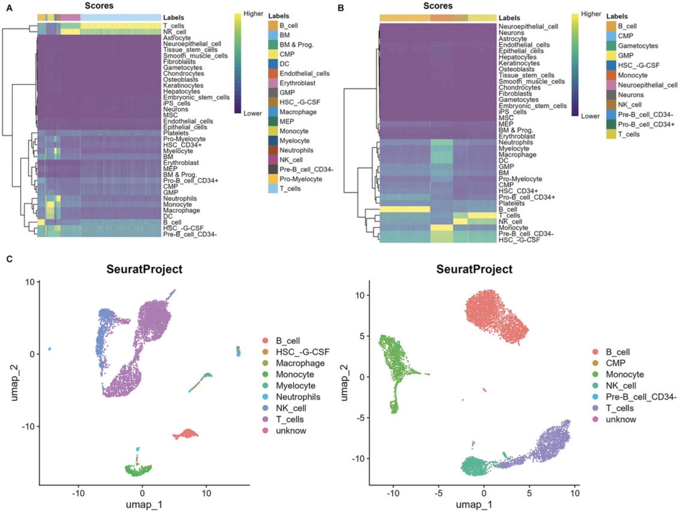
3.Visualize the cell type annotation.

Note

The plotScoreHeatmap and the DimPlot functions in the SingleR and Seurat packages, respectively, can be useful in visualizing cell types in the data. The below code has been provided to illustrate the cell annotations. The expected results are shown in Figure 12.

# Cell annotation scores

p_cell_1 <- plotScoreHeatmap(subset_demo_seurat_1@misc$SingleR_results,

show_colnames = F)

p_cell_2 <- plotScoreHeatmap(subset_demo_seurat_2@misc$SingleR_results,

show_colnames = F)

func_save_images(image.object = list(p_cell_1,

p_cell_2),

image.name = c("Subset - heatmap of singleR annotation scores - demo 1",

"Subset - heatmap of singleR annotation scores - demo 2"),

image.path = "Protocol 4 output",

h = 5,

w = 7,

r = 300,

isHeatmap = F

)

# Display cells in UMAP plot

p_cell_3 <- Seurat::DimPlot(subset_demo_seurat_1,

group.by = "cell_type") +

ggtitle(Project(subset_demo_seurat_1))

p_cell_4 <- Seurat::DimPlot(subset_demo_seurat_2,

group.by = "cell_type") +

ggtitle(Project(subset_demo_seurat_2))

patchwork::wrap_plots(p_cell_3 +

p_cell_4)

func_save_images(image.object = list(patchwork::wrap_plots(p_cell_3 +

p_cell_4)),

image.name = "Subset - UMAP group by cell type",

image.path = saveTo,

h = 5,

w = 13,

r = 300,

isHeatmap = F

)

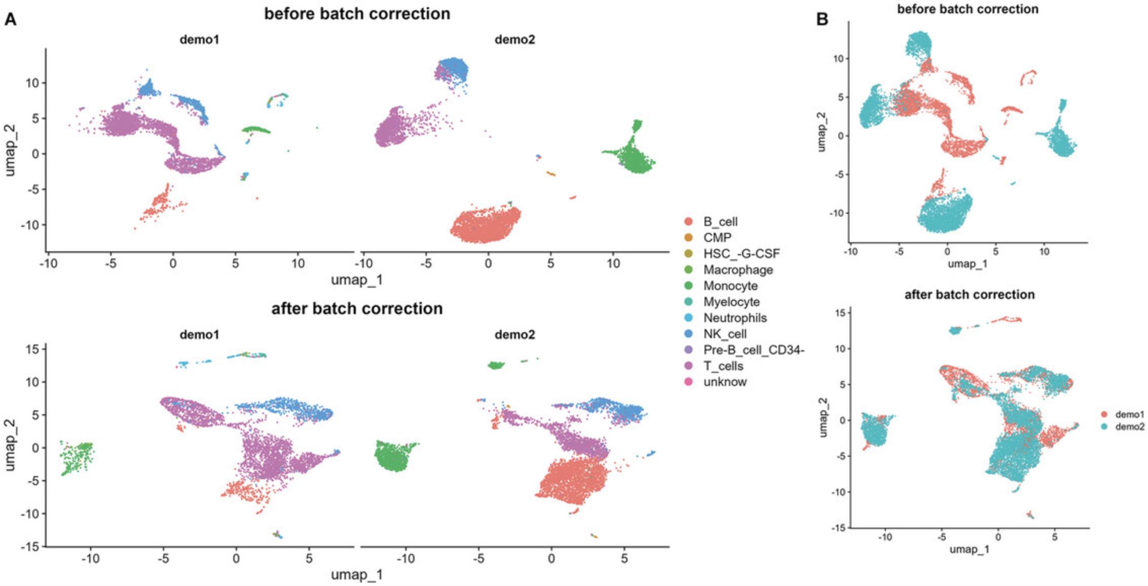
Cell annotation using SingleR. (A) and (B) Heatmaps showing cell type prediction scores for the demo exp 1 and demo exp 2 datasets, respectively. (C) UMAP plots with clusters highlighted by cell type.

4.Merge datasets and remove batch effect.

Note

When multiple datasets from different sequencing runs and/or sources are used, batch effects arise, resulting in misinterpretation of the true biological variance (Haghverdi et al., 2018). The combination of SelectIntegrationFeatures, FindIntegrationAnchors, and IntegrateData functions in the Seurat package can merge multiple datasets with batch effect correction. However, these functions are not efficient when handling large datasets. Instead, we propose using the harmony package, which can remove batch effects on large datasets and is integrated with Seurat objects.

Note

As an illustration here, we merge two demo datasets into one Seurat object and then apply harmony to remove batch effects. Therefore, in this step, we achieve harmonization of two datasets using the func_harmony function.

# Merge experiments

levels(subset_demo_seurat_1$orig.ident) <- "demo1"

levels(subset_demo_seurat_2$orig.ident) <- "demo2"

subset_demo_combined <- merge(subset_demo_seurat_1,

y = subset_demo_seurat_2,

add.cell.ids = c("demo1",

"demo2"),

project = "demo")

# Cluster cells

subset_demo_combined <- func_quick_process(subset_demo_combined)

# Check batch effect

p_cell_5 <- Seurat::DimPlot(subset_demo_combined,

reduction = "umap",

group.by = "orig.ident") +

ggtitle("before batch correction")

p_cell_6 <- Seurat::DimPlot(subset_demo_combined,

reduction = "umap",

split.by = "orig.ident",

group.by = "cell_type") +

ggtitle("before batch correction")

# Use Harmony to negate the batch effect

# type ?harmony in the Rstudio console to find out more information

func_harmony<- function(seuratObj,

rna_pc_num = 15,

rna_reduction_res = 0.8)

{

Seurat::DefaultAssay(seuratObj) <- "RNA"

seuratObj <- seuratObj %>%

Seurat::NormalizeData() %>%

Seurat::FindVariableFeatures(.,

selection.method = "vst",

nfeatures = 500)

seuratObj <- Seurat::ScaleData(seuratObj,

verbose = FALSE)

seuratObj <- Seurat::RunPCA(seuratObj,

npcs = rna_pc_num,

verbose = FALSE)

seuratObj <- harmony::RunHarmony(seuratObj,

"orig.ident")

seuratObj <- Seurat::RunUMAP(seuratObj,

reduction = "harmony",

dims = 1:rna_pc_num)

seuratObj <- Seurat::FindNeighbors(seuratObj,

reduction = "harmony",

dims = 1:rna_pc_num)

seuratObj <- Seurat::FindClusters(seuratObj,

resolution = rna_reduction_res)

seuratObj <- Seurat::BuildClusterTree(seuratObj)

# Return Seurat object

return(seuratObj)

} # end of func_harmony function

# Perform batch effect correction

subset_demo_combined <- func_harmony(subset_demo_combined,

rna_pc_num = 15,

rna_reduction_res = 0.8)

Note

The harmonized data are contained in the object subset_demo_combined. The below code uses the Dimplot function in Seurat to show the effect of harmony and is used to generate Figure 13.

p_cell_7 <- Seurat::DimPlot(subset_demo_combined,

reduction = "umap",

group.by = "orig.ident") +

ggtitle("after batch correction")

p_cell_8 <- Seurat::DimPlot(subset_demo_combined,

reduction = "umap",

split.by = "orig.ident",

group.by = "cell_type") +

ggtitle("after batch correction")

patchwork::wrap_plots(p_cell_5 +

p_cell_7)

func_save_images(image.object = list(patchwork::wrap_plots(p_cell_5 +

p_cell_7) +

plot_layout(guides = 'collect')),

image.name = "Subset - batch effect removal",

image.path = "Protocol 4 output",

h = 5,

w = 11,

r = 300,

isHeatmap = F

)

patchwork::wrap_plots(p_cell_6 +

p_cell_8)

func_save_images(image.object = list(patchwork::wrap_plots(p_cell_6 +

p_cell_8) +

plot_layout(guides = 'collect')),

image.name = "Subset - batch effect removal - split",

image.path = "Protocol 4 output",

h = 8,

w = 11,

r = 300,

isHeatmap = F

)

UMAP plots showing merged datasets before and after batch effect correction using harmony. (A) Merged datasets split by sample, with cell types highlighted. (B) Merged datasets of demo exp 1 and demo exp 2 clustered and highlighted by dataset.

5.Find doublets with DoubletFinder.

Note

It is important to identify doublets in scRNA-seq data for two reasons: 1) artificially created doublets do not represent biologically relevant events and may falsely appear as new cell types, and 2) they can falsely represent true cell clusters.

Note

For more information and a comparison of doublet-detecting methods, see Xi & Li (2021). In this protocol, DoubletFinder is used for doublet identification (McGinnis et al., 2019). The doublet rates for the BD Rhapsody system at different cell load numbers are provided by the manufacturer (Fig. 2). We use this set of numbers to create a linear model. In this step, the func_get_doublets function is used to calculate the doublet rate based on the cell number of the dataset and uses the computed doublet rate as the reference for the DoubletFinder simulation. Additionally, in this step, doublets are not excluded from the dataset but are rather labeled as “doublets” in the metadata.

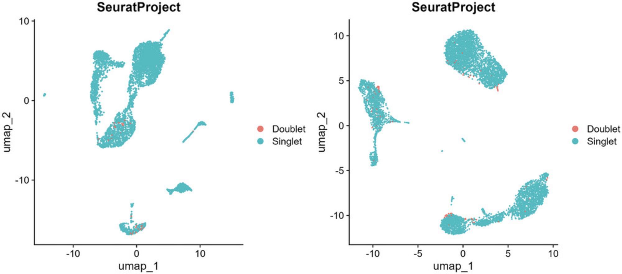
# Find doublets

# BD provided doublet rates with different cell load numbers

rhapsody_doublet_rate <- data.frame(

"cell_num" = c(100,500,1000*(1:20)),

"rate" = c(0, 0.1, 0.2, 0.5, 0.7, 1,

1.2, 1.4, 1.7, 1.9, 2.1,

2.4, 2.6, 2.8, 3.1, 3.3,

3.5, 3.8, 4, 4.2, 4.5 , 4.7))

# Build a linear model to calculate theoretical doublet rate

model_rhap <- lm(rate ∼ cell_num,

rhapsody_doublet_rate)

# define function

func_get_doublets <- function(seuratObj,

est_doublet_model = model_rhap,

pc = 1:15) # number of PC components to be used

{

DefaultAssay(seuratObj) <- "RNA"

# Find pK values

sweep.res.list <- paramSweep_v3(seuratObj,

PCs = pc,

sct = F)

sweep.stats <- summarizeSweep(sweep.res.list,

GT = FALSE)

bcmvn <- find.pK(sweep.stats)

pK_bcmvn <- bcmvn$pK[which.max(bcmvn$BCmetric)] %>%

as.character() %>%

as.numeric()

# estimate doublet rate based on cell number

DoubletRate = predict(est_doublet_model,

data.frame(cell_num = dim(seuratObj)[2]))/100

nExp_poi <- round(DoubletRate*ncol(seuratObj))

seuratObj <- doubletFinder_v3(seuratObj,

PCs = pc,

pN = 0.25,

pK = pK_bcmvn,

nExp = nExp_poi,

reuse.pANN = F,

sct = F)

temp1 <- grepl("DF.classifications",

colnames(seuratObj@meta.data),

ignore.case = T)

colnames(seuratObj@meta.data)[temp1] <- "doublet_check"

seuratObj$doublet_check <- seuratObj$doublet_check

# return output

return(seuratObj)

} # end of function

# use function to find doublets

subset_demo_seurat_1 <- func_get_doublets(subset_demo_seurat_1,

pc = 1:15)

subset_demo_seurat_2 <- func_get_doublets(subset_demo_seurat_2,

pc = 1:15)

Note

The below code uses the Dimplot function in Seurat and creates a UMAP of doublets or singlets identified (Fig. 14).

# Visualize the result

p_cell_9 <- DimPlot(subset_demo_seurat_1,

group.by = "doublet_check") +

ggtitle(Project(subset_demo_seurat_1))

p_cell_10 <- DimPlot(subset_demo_seurat_2,

group.by = "doublet_check") +

ggtitle(Project(subset_demo_seurat_2))

patchwork::wrap_plots(p_cell_9 +

p_cell_10)

func_save_images(image.object = list(patchwork::wrap_plots(p_cell_9 +

p_cell_10)),

image.name = "Subset - doublets",

image.path = saveTo,

h = 5,

w = 11,

r = 300,

isHeatmap = F

)

UMAP of demo exp 1 and demo exp 2 highlighted by doublets or singlets identified by DoubletFinder. The left panel shows the doublets for demo exp 1, and the right panel shows doublets for demo exp 2.

6.Find marker genes.

Note

In this step, we use the func_get_marker_genes function to identify the differentially expressed genes (DGEs) that define each of the clusters and cell types. Once all DGEs are identified, we select only the top five DGEs that define each cluster/cell type. Although the Seurat package has the function Seurat::FindAllMarkers to calculate DGEs, the algorithm is relatively time consuming. Therefore, it is recommended to use the function RunPrestoAll in the SeuratWrappers package.

Note

This approach can trigger a warning when the groups being compared have less than three cells within a group. Grouping populations of cells with low cell numbers can avoid the warning; however, this makes data interpretation harder.

Note

The below code creates the func_get_marker_genes function and applies it to the already-subsetted demo exp 1 and demo exp 2 data.

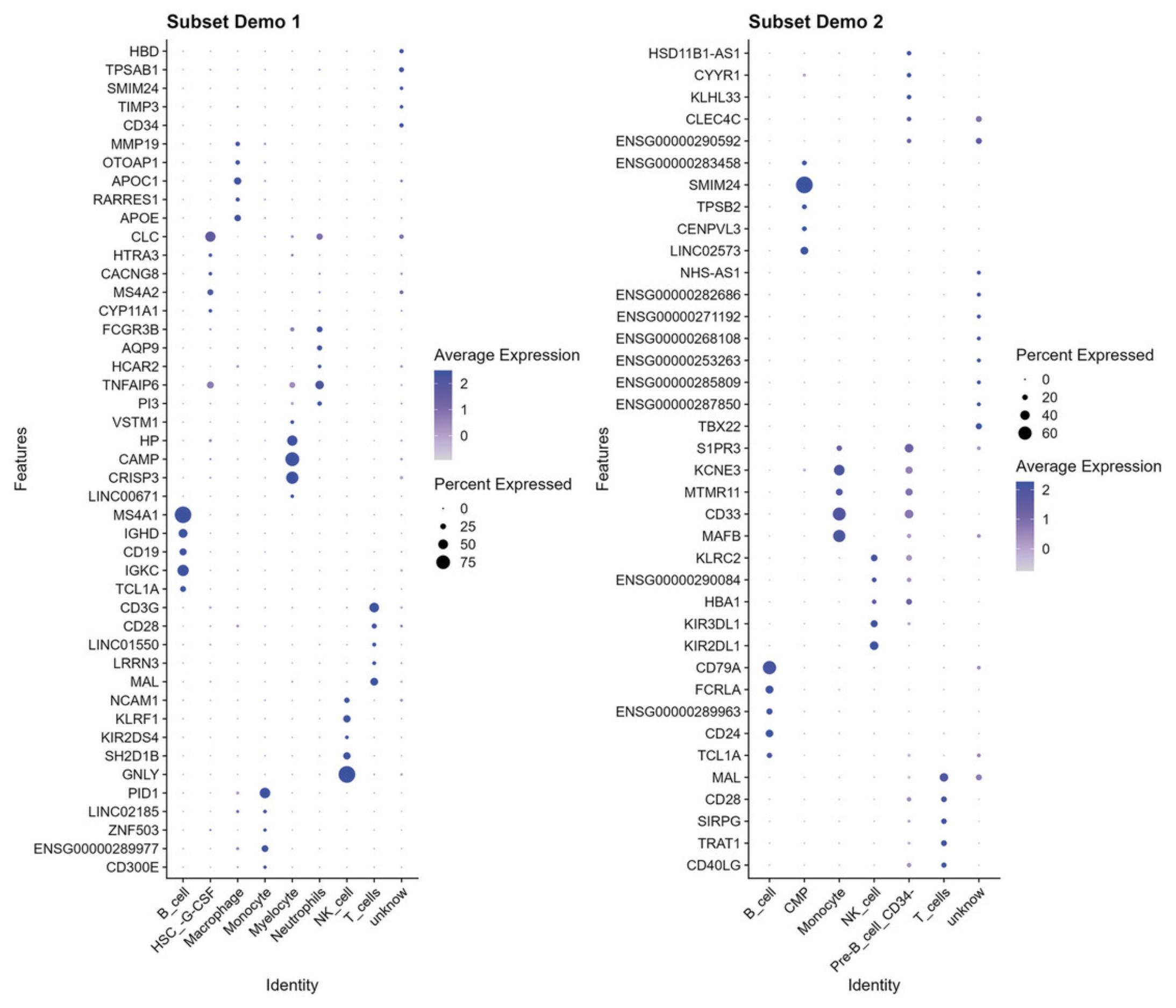
# Build function

func_get_marker_genes <- function(input_seurat,

p_adj_cutoff = 0.05,

log2FC_cutoff = 1,

view_top_X_genes = 5)

{

# Find marker genes for each cluster group against the rest

Seurat::Idents(input_seurat) <- "seurat_clusters"

cluster_DGE <- SeuratWrappers::RunPrestoAll(input_seurat,

assay = "RNA",

only.pos = FALSE,

verbose = FALSE)

# Find marker genes for each cell type against the rest

Seurat::Idents(input_seurat) <- "cell_type"

Cell_type_DGE <- SeuratWrappers::RunPrestoAll(input_seurat,

assay = "RNA",

only.pos = FALSE,

verbose = FALSE)

# example of taking the top X genes in each DGE group and removing the duplicates

cluster_DGE <- cluster_DGE[abs(cluster_DGE$avg_log2FC) > log2FC_cutoff &

cluster_DGE$p_val_adj < p_adj_cutoff, ]

Cell_type_DGE <- Cell_type_DGE[abs(Cell_type_DGE$avg_log2FC) > log2FC_cutoff &

Cell_type_DGE$p_val_adj < p_adj_cutoff, ]

top_genes_cluster <- cluster_DGE %>%

group_by(cluster)%>%

slice_max(n = view_top_X_genes,

order_by = avg_log2FC) %>%

dplyr::pull(gene) %>%

unique()

top_genes_type <- Cell_type_DGE %>%

group_by(cluster)%>%

slice_max(n = view_top_X_genes,

order_by = avg_log2FC) %>%

dplyr::pull(gene) %>%

unique()

# return output as a list

return(list(DGEs_cluster = cluster_DGE,

DGEs_cell = Cell_type_DGE,

top_cluster_gene = top_genes_cluster,

top_cell_gene = top_genes_type))

} # end of function

# use function to get marker genes

subset_demo1_DGEs <- func_get_marker_genes(subset_demo_seurat_1,

p_adj_cutoff = 0.05,

log2FC_cutoff = 1,

view_top_X_genes = 5)

subset_demo2_DGEs <- func_get_marker_genes(subset_demo_seurat_2,

p_adj_cutoff = 0.05,

log2FC_cutoff = 1,

view_top_X_genes = 5)

To view the marker genes, use the code below for each dataset.

# display example results

subset_demo1_DGEs$top_cell_gene

"CD300E" "ENSG00000289977" "ZNF503""LINC02185" "PID1""GNLY" "SH2D1B" "KIR2DS4" "KLRF1" "NCAM1""MAL" "LRRN3" "LINC01550" "CD28" "CD3G" "TCL1A" "IGKC" "CD19" "IGHD" "MS4A1" "LINC00671" "CRISP3" "CAMP" "HP" "VSTM1" "PI3" "TNFAIP6" "HCAR2" "AQP9" "FCGR3B""CYP11A1" "MS4A2" "CACNG8" "HTRA3" "CLC" "APOE" "RARRES1" "APOC1" "OTOAP1" "MMP19" "CD34" "TIMP3" "SMIM24" "TPSAB1" "HBD"

# display example results

subset_demo2_DGEs$top_cell_gene

"CD40LG" "TRAT1" "SIRPG" "CD28" "MAL" "TCL1A" "CD24" "ENSG00000289963" "FCRLA" "CD79A" "KIR2DL1" "KIR3DL1" "HBA1" "ENSG00000290084" "KLRC2" "MAFB" "CD33" "MTMR11" "KCNE3" "S1PR3" "TBX22" "ENSG00000287850" "ENSG00000285809" "ENSG00000253263" "ENSG00000268108" "ENSG00000271192" "ENSG00000282686" "NHS-AS1" "LINC02573" "CENPVL3" "TPSB2" "SMIM24" "ENSG00000283458" "ENSG00000290592" "CLEC4C" "KLHL33" "CYYR1" "HSD11B1-AS1"

Note

The below code uses the Dotplot function in Seurat and creates a way to visualize both the expression level and the frequency of cells expressing the top five DGEs across all cell types identified in demo exp 1 and demo exp 2. Results are shown in Figure 15.

# visualise top genes on dotplot

p_cell_10 <- DotPlot(subset_demo_seurat_1,

features = subset_demo1_DGEs$top_cell_gene,

group.by = "cell_type") +

coord_flip() +

RotatedAxis() +

ggtitle("Subset Demo 1")

p_cell_11 <- DotPlot(subset_demo_seurat_2,

features = subset_demo2_DGEs$top_cell_gene,

group.by = "cell_type") +

coord_flip() +

RotatedAxis() +

ggtitle("Subset Demo 2")

patchwork::wrap_plots(p_cell_10 + p_cell_11)

func_save_images(image.object = list(patchwork::wrap_plots(p_cell_10 + p_cell_11)),

image.name = "Subset - top genes dot plot",

image.path = saveTo,

h = 12,

w = 14,

r = 300,

isHeatmap = F

)

Dot plots of demo exp 1 and demo exp 2 showing expression of top marker genes in the cell types identified.

7.Perform pseudotime and trajectory analysis.

Note

Algorithms have been developed to make use of gene expression changes to predict how cells migrate from one functional “state” to another. To study cellular dynamics, monocle3 and slingshot are used. For a comparison of different single-cell trajectory inference methods, see Saelens et al. (2019). Both packages return a computed pseudotime for each cell, where pseudotime is defined by what stage the cell is in.

Note

For monocle3 analysis, we load and run the func_monocle3 function to reconstruct single-cell trajectories using monocle3. This R package does not accept a Seurat object as a valid input format; therefore, the Seurat object needs to be converted into a SingleCellExperiment (SCE) class. After the format conversion, monocle3 clusters the cells with cluster_cells and then orders cells with learn_graph and order_cells. Set parameter use_partition to TRUE or FALSE within the learn_graph function to use a single graph to learn across all partitions or to create a disjoint graph for each partition. The program requires “root” cells or cells at an early stage as a starting point for the calculation. There are stem cells or CD34+ cells in the demo data (see results from step 2, regarding cell type annotation with SingleR), which are used as the root cells for the analysis. This demo data are annotated with reference data from the “Human Primary Cell Atlas” using the R package “celldex.” Cells annotated with cell types containing any of the words “CMP, GMP, HSC, CD34, stem, and iPS” are defined as root cells (these are examples for this specific analysis; please define root cells that are biologically relevant for your experiment). It is important to note that the cell type naming convention is not the same across all reference datasets. Inspecting the annotation results before determining the root cells for monocle3 analysis is also essential. Following the use of monocle3 to determine cell trajectories, the data are then written back into a Seurat object. This analysis is only performed on demo exp 1.

# Monocle3 trajectory analysis

# Define function

func_monocle3 <- function(input_seurat,

rna_pc_num = 50)

{

# covert Seurat to SingleCellExperiment object

demo_cds <- SeuratWrappers::as.cell_data_set(input_seurat)

rowData(demo_cds)$gene_short_name <- rownames(input_seurat)

demo_cds <- preprocess_cds(demo_cds,

num_dim = rna_pc_num)

demo_cds <- monocle3::reduce_dimension(demo_cds)

demo_cds <- monocle3::cluster_cells(cds = demo_cds,

cluster_method = "louvain")

# Change parameter use_partition to TRUE to learn disjoint graph in each partition

demo_cds <- monocle3::learn_graph(demo_cds,

use_partition = FALSE)

Seurat::Idents(input_seurat) <- "cell_type"

# This is just an example. Please define root cells that are biologically

# correct for your experiment.

# Note: if ids is an empty object, then this function may generate error.

# You can use this line instead:

# demo_cds <- monocle3::order_cells(demo_cds, reduction_method = "UMAP")

# and remove the following three lines,

# "ids <- ..",

# "root_id <- .."

# "demo_cds <- .."

# for more information, please visit

# https://cole-trapnell-lab.github.io/monocle3/docs/trajectories/

ids <- unique(input_seurat$cell_type) %>%

.[grep(paste("CMP",

"GMP",

"HSC",

"CD34",

"stem",

"iPS",

sep = "|"),

ignore.case = T)]

root_id <- colnames(subset(input_seurat,

idents = ids))

demo_cds <- monocle3::order_cells(demo_cds,

reduction_method = "UMAP",

root_cells = root_id)

colData(demo_cds)$m3_pseudotime <- pseudotime(demo_cds)

# return Seurat object

return(demo_cds)

}

# use function to get results

subset_demo_cds_1 <- func_monocle3(subset_demo_seurat_1,

rna_pc_num = 50)

subset_demo_seurat_1 <- Seurat::AddMetaData(

object = subset_demo_seurat_1,

metadata = pseudotime(subset_demo_cds_1),

col.name = "m3_pseudotime"

)

_The code below uses various plotting tools to display the results of monocle3 analysis (_Fig. 16 ).

# Display results

# Check monocle3 trajectory

p_m3_pseudo_all <- plot_cells(subset_demo_cds_1,

color_cells_by = "pseudotime",

label_cell_groups=FALSE,

label_leaves=FALSE,

label_branch_points=FALSE,

graph_label_size=1.5) +

ggtitle("All cells (UMAP done on Monocle3)")

p_m3_pseudo_tag1 <- plot_cells(subset_demo_cds_1[, grepl("SampleTag01_hs",

colData(subset_demo_cds_1)$smk,

ignore.case=TRUE)],

color_cells_by = "pseudotime",

label_cell_groups=FALSE,

label_leaves=FALSE,

label_branch_points=FALSE,

graph_label_size=1.5) +

ggtitle("SampleTag01_hs (UMAP done on Monocle3)")

p_m3_pseudo_tag2 <- plot_cells(subset_demo_cds_1[, grepl("SampleTag02_hs",

colData(subset_demo_cds_1)$smk,

ignore.case=TRUE)],

color_cells_by = "pseudotime",

label_cell_groups=FALSE,

label_leaves=FALSE,

label_branch_points=FALSE,

graph_label_size=1.5) +

ggtitle("SampleTag02_hs (UMAP done on Monocle3)")

wrap_plots(p_m3_pseudo_all +

p_m3_pseudo_tag1 +

p_m3_pseudo_tag2) +

func_save_images(image.object = list(wrap_plots(p_m3_pseudo_all +

p_m3_pseudo_tag1 +

p_m3_pseudo_tag2)),

image.name = "Subset - monocle3 trajectory",

image.path = saveTo,

h = 5,

w = 15,

r = 300,

isHeatmap = F

)

# Check pseudotime for different sample tags

Idents(subset_demo_seurat_1) <- "smk"

p_m3_celltype <- ggplot(subset(subset_demo_seurat_1,

idents = c("SampleTag01_hs",

"SampleTag02_hs"))@meta.data,

aes(x = m3_pseudotime,

y = cell_type,

colour = cell_type)) +

geom_point() +

geom_jitter(width = 0.1,

height = 0.2) +

theme_gray() +

theme(legend.position = "none") +

facet_grid(. ∼ smk )

p_m3_celltype

func_save_images(image.object = list(p_m3_celltype),

image.name = "Subset - monocle3 pseudotime split by smk",

image.path = saveTo,

h = 5,

w = 11,

r = 300,

isHeatmap = F

)

# Check pseudotime in Seuart UMAP embeddings

Idents(subset_demo_seurat_1) <- "smk"

p_m3_pseudo_umap <- Seurat::FeaturePlot(subset(subset_demo_seurat_1,

idents = c("SampleTag01_hs",

"SampleTag02_hs")),

features = "m3_pseudotime") +

ggtitle("All cells") &

scale_color_viridis_c("m3_pseudotime")

p_m3_pseudo_umap

func_save_images(image.object = list(p_m3_pseudo_umap),

image.name = "Subset - monocle3 pseudotime (in Seurat) all cells",

image.path = saveTo,

h = 5,

w = 6,

r = 300,

isHeatmap = F

)

p_m3_pseudo_umap_split <- Seurat::FeaturePlot(subset(subset_demo_seurat_1,

idents = c("SampleTag01_hs",

"SampleTag02_hs")),

features = "m3_pseudotime",

split.by = "smk") &

theme(legend.position="right") &

scale_color_viridis_c("m3_pseudotime")

p_m3_pseudo_umap_split

func_save_images(image.object = list(p_m3_pseudo_umap_split),

image.name = "Subset - monocle3 pseudotime (in Seurat) split by smk",

image.path = saveTo,

h = 5,

w = 13,

r = 300,

isHeatmap = F

)

# Display Cell types in Seurat UMAP

p_dim_umap <- Seurat::DimPlot( subset(subset_demo_seurat_1,

idents = c("SampleTag01_hs",

"SampleTag02_hs")),

group.by = "cell_type",

split.by = "smk")

p_dim_umap

func_save_images(image.object = list(p_dim_umap),

image.name = "Subset - monocle3 cell type check",

image.path = saveTo,

h = 5,

w = 11,

r = 300,

isHeatmap = F

)

# Display pseudotime vs gene expression

p_pseudo_gene_1 <- FeatureScatter(subset(subset_demo_seurat_1,

idents = c("SampleTag01_hs",

"SampleTag02_hs")),

feature1 = "m3_pseudotime",

feature2 = "CD8A",

group.by = "smk") +

ggtitle("")

p_pseudo_gene_2 <- FeatureScatter(subset(subset_demo_seurat_1,

idents = c("SampleTag01_hs",

"SampleTag02_hs")),

feature1 = "m3_pseudotime",

feature2 = "CD19",

group.by = "smk") +

ggtitle("")

p_pseudo_gene_3 <- FeatureScatter(subset(subset_demo_seurat_1,

idents = c("SampleTag01_hs",

"SampleTag02_hs")),

feature1 = "m3_pseudotime",

feature2 = "NKG7",

group.by = "smk") +

ggtitle("")

p_pseudo_gene <- wrap_plots(p_pseudo_gene_1 +

p_pseudo_gene_2 +

p_pseudo_gene_3) +

plot_layout(guides = "collect")

p_pseudo_gene

func_save_images(image.object = list(p_pseudo_gene),

image.name = "Subset - monocle3 pseudotime vs gene expression",

image.path = saveTo,

h = 5,

w = 11,

r = 300,

isHeatmap = F

)

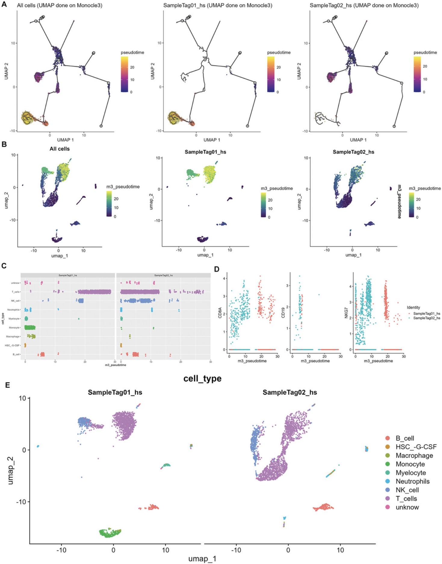
monocle3 analysis of a pooled sample where SampleTag01_hs were non-treated and SampleTag02_hs were activated in the presence of CD3/CD28 for 24 hr. (A) UMAP calculated by monocle3 showing the lineage trajectory and pseudotime. (B) UMAP from Seurat highlighted by pseudotime. (C) Pseudotime comparison between SampleTag01_hs and SampleTag02_hs across all cell types. (D) Scatter plots of gene expression against pseudotime. (E) UMAP from Seurat object subset_demo_seurat_1 first split by sample tag and then highlighted by cell type.

In slingshot analysis, we load and run the func_slingshot _function to reconstruct single-cell trajectories using slingshot. Slingshot uses a different approach compared to monocle3, as it calculates pseudotime with or without definition of a group of root cells as the beginning point. It performs two main steps to calculate pseudotime: 1) defines lineage structure via a cluster-based Minimum Spanning Tree (MST) and 2) fits simultaneous principal curves to the lineage (_Street et al. , 2018 ). We will use the same dataset used in the monocle3 analysis. Root cells are defined the same way as in monocle3 analysis. These cells are renamed to “start_clus.” The Seurat objects are then converted into an SCE class and passed into slingshot for pseudotime calculation.

# slingshot pseudotime analysis

# Define function

func_slingshot <- function(input_seurat)

{

# group cells at early states as start_clus

# This is just an example. Please define root cells that are biologically

# correct for your experiment.

# Note: if ids is an empty object, then this function may generate error.

# You can use this line instead:

# demo_sce <- slingshot::slingshot(demo_sce,

# clusterLabels = "cell_type",

# reducedDim = "PCA",

# allow.breaks = F)

# and remove the following four lines, "Seurat::Idents(input_seurat) <- ..",

# "ids <- ..."

# "input_seurat$cell_type <- .." and

# "input_seurat$cell_type[input_seurat$cell_type %in% ids] <- .."

# for more information, please visit

# http://www.bioconductor.org/packages/release/bioc/vignettes/slingshot/inst/doc/vignette.html

Seurat::Idents(input_seurat) <- "cell_type"

ids <- unique(input_seurat$cell_type) %>%

.[grep(paste("CMP",

"GMP",

"HSC",

"CD34",

"stem",

"iPS",

sep = "|"),

ignore.case = T)]

input_seurat$cell_type[input_seurat$cell_type %in% ids] <- "start_clus"

# convert Seurat to SingleCellExperiment class

demo_sce <- Seurat::as.SingleCellExperiment(input_seurat)

# Perform slingshot analysis

temp <- tryCatch(

{

# PCA, tSNE and UMAP are all accepted for slingshot analysis.

# However, PCA has more dimensions. Hence, it's recommended by Slingshot Author.

# Subset first 6 PC components

reducedDim(demo_sce,

type = "PCA",

WithDimnames = TRUE) <- reducedDim(demo_sce,

type = "PCA")[, 1:6]

demo_sce <- slingshot::slingshot(demo_sce,

clusterLabels = "cell_type",

start.clus = "start_clus",

reducedDim = "PCA",

allow.breaks = F)

error = function(e){

# if there is an issue with PC selection, switch reduction method to UMAP

demo_sce <- slingshot::slingshot(demo_sce,

clusterLabels = "cell_type",

start.clus = "start_clus",

reducedDim = "UMAP",

allow.breaks = F)

}

)

# return SCE object

return(temp)

} # end of function

# use function to get results

subset_demo_slingshot_1 <- func_slingshot(subset_demo_seurat_1)

pt_lineages <- slingshot::slingPseudotime(subset_demo_slingshot_1)

# add Slingshot results to the input Seurat object

lineages <- sapply(slingLineages(colData(subset_demo_slingshot_1)$slingshot),

paste,

collapse = " -> ")

subset_demo_seurat_1@meta.data[lineages] <- pt_lineages

_The code below demonstrates the slingshot analysis results (_Fig. 17 ).

# display results

# visualization

# display every lineage pseudotime

name_lineage <- colnames(subset_demo_seurat_1@meta.data)[grepl("->",

colnames(subset_demo_seurat_1@meta.data))]

p_ss_1 <- list()

Idents(subset_demo_seurat_1) <- "smk"

for (i in name_lineage) {

p_ss_1[[i]] <- Seurat::FeaturePlot(subset(subset_demo_seurat_1,

idents = c("SampleTag01_hs",

"SampleTag02_hs")),

features = i, split.by = "smk") &

theme(legend.position="top") &

scale_color_viridis_c()

}

wrap_plots(p_ss_1,

ncol = 1)

func_save_images(image.object = list(wrap_plots(p_ss_1,

ncol = 1)),

image.name = "Subset - slingshot pseudotime (in Seurat) split by smk",

image.path = saveTo,

h = 30,

w = 18,

r = 300,

isHeatmap = F

)

# Display lineage curves

color <- colorRamps::blue2green2red(length(unique(subset_demo_seurat_1$cell_type)))

names(color) <- unique(subset_demo_seurat_1$cell_type)

tiff(filename = paste(saveTo,

"Subset - slingshot lineages.tiff",

sep = "/"),

compression = "lzw",

width = 6,

height = 5,

units = "in",

res = 300)

{

par(mar = c(6,4,6,12) + 0.1,

xpd = T)

plot(reducedDim(subset_demo_slingshot_1 , "PCA"),

pch=16,

cex = 0.5,

col = color[as.character(subset_demo_seurat_1$cell_type)])

title("Slingshot Lineages")

legend("right",

legend = names(color),

fill = color,

inset = c(-0.7,0))

lines(SlingshotDataSet(colData(subset_demo_slingshot_1)$slingshot),

lwd = 2,

col = 'black',

type = 'lineages')

}

dev.off()

# Check pseudotime for different sample tags

p_ss_celltype <- list()

Idents(subset_demo_seurat_1) <- "smk"

for (i in name_lineage) {

p_ss_celltype[[i]] <- ggplot(subset(subset_demo_seurat_1,

idents = c("Multiplet",

"Undetermined"),

invert = T)@meta.data,

aes(x = .data[[i]],

y = cell_type,

colour = cell_type)) +

geom_point() +

geom_jitter(width = 0.1,

height = 0.2) +

theme_gray() +

theme(legend.position = "none") +

facet_grid(. ∼ smk )

}

wrap_plots(p_ss_celltype,

ncol = 2)

func_save_images(image.object = list(wrap_plots(p_ss_celltype,

ncol = 1)),

image.name = "Subset - slingshot pseudotime split by smk",

image.path = saveTo,

h = 16,

w = 8,

r = 300,

isHeatmap = F

)

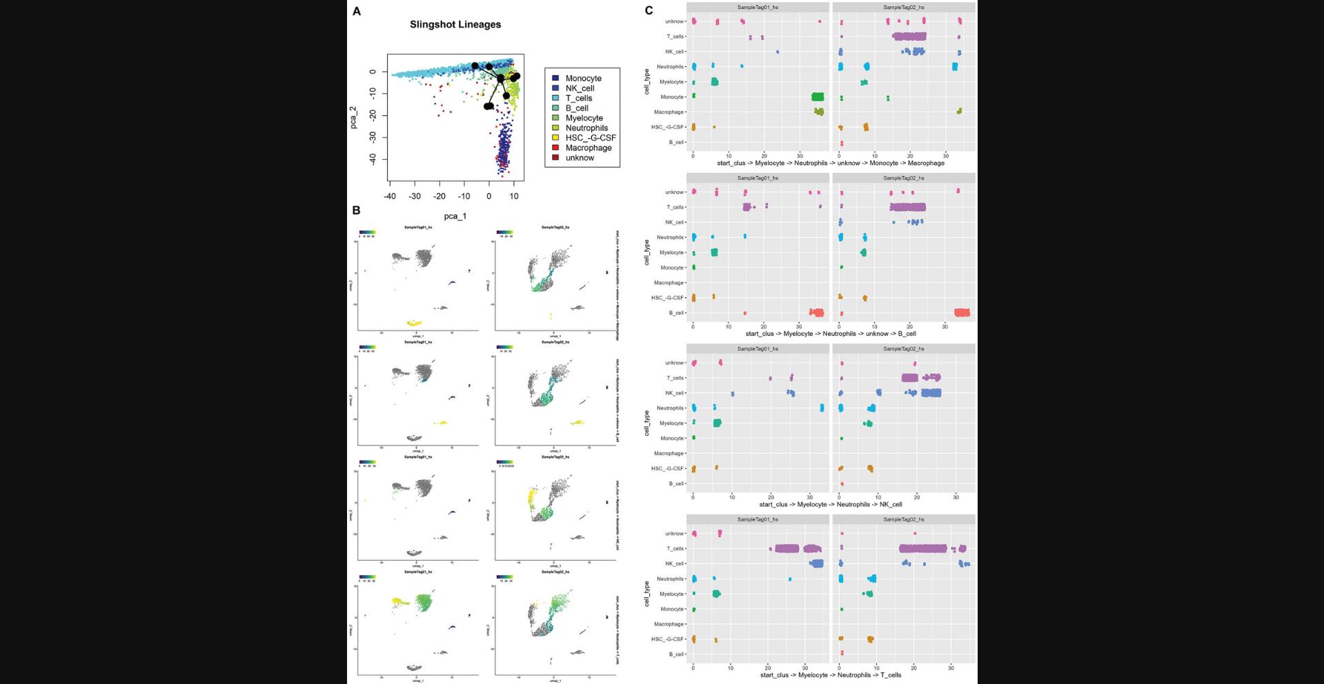
Pseudotime calculation by slingshot. (A) Cell lineages calculated by slingshot displayed on a PCA plot. (B) and (C) Pseudotime comparison between SampleTag01_hs and SampleTag02_hs across all lineage paths and cell types, respectively.

8.Evaluate cell-cell communication.

_In this step, we evaluate cell-cell signaling or communication, which can be assessed by analyzing the interactions between ligands and receptors. CellPhoneDB (_Efremova et al. , 2020 _) and CellChat (_Jin et al. , 2021 ) quantify cell-cell interaction by utilizing network analysis and pattern recognition methods.

CellPhoneDB requires Anaconda and is outside the R environment; therefore, it is outside the scope of this protocol. Nevertheless, we provide details for execution in the Supporting Information provided with this article, entitled “** Protocol Supp CellphoneDB.Rmd** ” and “** Cell-cell communication analysis with CellphoneDB.docx** .”

For CellChat, we load and run the func_cellchat function in order to identify cell-cell interactions. CellChat is similar to CellPhoneDB in regard to the heteromeric complex approach but differs from it in database curation, which also includes other factors, including, but not limited to, soluble agonists and antagonists. Seurat objects can be input into the package directly, without format conversion. In the following example, we use the cell type to group cells, and cell-cell interactions are quantified among these groups. The results are saved as a .csv file, which can be visualized by another package called InterCellar (see Basic Protocol Basic Protocol 6 ).

Cell-cell communication is calculated for both demo exp 1 and demo exp 2.

# CellChat cell-cell communication analysis

# create function

func_cellchat <- function(input_seurat,

output_name)

{

# use cell type to grouop cells

cc.object <- CellChat::createCellChat(object = input_seurat,

group.by = "cell_type")

# if it is a mouse tissue, use CellChatDB.mouse

cc.object@DB <- CellChat::CellChatDB.human

cc.object <- CellChat::subsetData(cc.object)

cc.object <- CellChat::identifyOverExpressedGenes(cc.object)

cc.object <- CellChat::identifyOverExpressedInteractions(cc.object)

# cc.object <- CellChat::projectData(cc.object, PPI.human)

cc.object <- CellChat::computeCommunProb(cc.object,

population.size = T,

raw.use = T)

cc.object <- CellChat::computeCommunProbPathway(cc.object)

cc.object <- CellChat::aggregateNet(cc.object)

output <- CellChat::subsetCommunication(cc.object,

slot.name = "net")

# Save the curated data to local drive

temp_folder <- paste(saveTo,

"CellChat output",

sep = "/")

ifelse(!dir.exists(file.path(temp_folder)),

dir.create(file.path(temp_folder)), FALSE)

write.csv(x = output,

file = paste(temp_folder,

paste0(output_name,".csv"),

sep = "/"))

} # end of function

# use function to export files

# parameter "output_name" for function func_cellchat can any string, e.g. output_name <- "PBMCs_1".

# Here, Seurat project names are used.

func_cellchat(input_seurat = subset_demo_seurat_1,

output_name = Project(subset_demo_seurat_1))

func_cellchat(input_seurat = subset_demo_seurat_2,

output_name = Project(subset_demo_seurat_2))

# Save Seurat objects to local drive

save(subset_demo_seurat_1,

subset_demo_seurat_2,

subset_demo1_DGEs,

subset_demo2_DGEs,

subset_demo_combined,

subset_demo_cds_1,

subset_demo_slingshot_1,

file = paste(saveTo,

"subsetted demo Seurat objects (advanced analysis).RData", sep = "/")

)

Basic Protocol 5: CONVERTING DATA TO FLOW CYTOMETRY STANDARD (FCS) FORMAT

In line with the principles of genomic cytometry, single-cell genomics should be more concerned with cellular characterization than with analyzing the genome alone. As such, the data produced in many BD Rhapsody experiments contain not just RNA information but also protein expression information. Regardless of the reporter molecule used to detect and quantify protein expression, the data from AbSeq can be visualized in the same way as for fluorescent and mass cytometry.

This protocol aims to build a bridge to connect scRNA-seq to cytometry in terms of traditional bi-variant cell gating using the more traditional cytometric gating tools to facilitate understanding. Therefore, biologists who are not familiar with programming do not need to master R or Python to perform basic single cell–based exploration of protein and/or RNA expression levels.

The script stores data in .FCS format, and the files can be analyzed with open-source software such as R and Python or commercial software such as FlowJo and FCS Express. Here, we demonstrate how to convert an oligo-ab matrix and gene expression matrix into a .FCS file. This protocol works for any scRNA-seq data that are in Seurat format, even if the data are not preprocessed.

To retain relevant information, the script exports data that include the following:

1.Protein expression on each cell 2.PCA/UMAP/T-sne coordinates 3. Cell clusters 4. Sample tag identities 5. Marker genes and user-selected genes in the form of normalized RNA read counts 6. MT gene expression percentage for each cell 7. UMI (nCount_RNA) counts per cell 8. Detectable gene count (nFeature_RNA) per cell.

Relevance

Cytometrists are familiar with analysis of FCS-formatted data using a graphical user interface (GUI) such as FlowJo, FCS Express, and other software packages. With this familiarity comes an ability to manually curate and interrogate the data. The capability to easily do this using a GUI reduces the need to code and makes data analysis available to more people. As FlowJo and FCS Express have integrated graphing tools, the results can easily be shared and incorporated into visual presentations.

Current Limitations

The FCS format is a data table that includes metadata associated with user- and instrument-derived experimental data. This script can produce data in .FCS format, but current FCS reader software may have limits on the number of rows and columns that can be reliably read. When dealing with large datasets, it is important to ensure that no data loss has occurred.

Necessary Resources

Software access : RStudio (≥2022.07.2 Build 576), R (≥4.2.1)
R packages :
- library(Seurat)
- library(flowCore)
Support files : N/A
Vignette dataset : Subsetted demo Seurat objects (advanced analysis).RData from Basic Protocol 4

1.Load data and create FCS conversion function.

In this step, we load the data produced in Basic Protocol Basic Protocol 4 and create the func_create_fcs function.

# load library

library(Seurat)

library(SeuratObject)

library(dplyr)

library(flowCore)

library(Biobase)

library(rstudioapi)

# set a seed to re-produce pseudorandom numbers

set.seed(99)

# Obtain the path of this rmarkdown file and assign it to object "get_path"

get_path <- dirname(rstudioapi::getSourceEditorContext()$path)

# Set "get_path" as Working Directory

setwd(get_path)

# Save images and data to this folder

saveTo <- "Protocol 5 output"

# load subsetted Seurat objects for Basic Protocol 4

load("Protocol 4 output/subsetted demo Seurat objects (advanced analysis).RData")

# parameter explanation

# @ para input_seurat

# Seurat object for data conversion

# @ para include_protein_assay_name

# name of protein assay if applicable

# @ para protein_data_type

# type of protein data. e.g. count

# @ para rna_genes_to_pull

# input can be output from FindAllMarkers() or FindMarkers() or a vector of genes

# @ para p_adj_cutoff, log2FC_cutoff and top_n_genes only are only application when

# rna_genes_to_pull is generated from FindAllMarkers() or FindMarkers()

# @ para extra_gene_list

# other genes to be included

# @ para rna_data_type

# type of rna data. e.g. count

# @ para meta_data_to_pull

# numeric data from the meta.data of the provided Seurat object

# e.g. nCount_RNA, nFeature_RNA

# @ para sample_id_to_pull

# categorical data from the meta.data of the provided Seurat object

# e.g. Sample_ID, seurat_clusters

# @ para embedding_to_pull

# which embedding to pull. e.g. pca, umap

# @ para add_jitter_to_which_meta

# add jitter effect to categorical meta data

# @ para outfile_name

# name for the output FCS file

# @ para save_path

# path to save the output FCS file

# example

# fsc_in_r <- func_create_fcs(input_seurat = cell_lines_qc,

# rna_genes_to_pull = c("LGALS1","MS4A1","TNF"),

# p_adj_cutoff = 0.05,

# log2FC_cutoff = 1,

# top_n_genes = 5,

# extra_gene_list = c("CD3D", "CD79A"),

# include_protein_assay_name = "AB",

# meta_data_to_pull = c("nCount_RNA",

# "nFeature_RNA",

# "percent.mt",

# "seurat_clusters",

# "doublet_check",

# "smk"),

# embedding_to_pull = c("umap", "adt.umap"),

# outfile_name = "export_fcs",

# add_jitter_to_which_meta = c("seurat_clusters", "smk"),

# sample_id_to_pull = c("smk", "doublet_check"),

# save_path = getwd())

# Create function

func_create_fcs <- function(input_seurat = NaN,

include_protein_assay_name = NaN,

protein_data_type = 'data',

rna_genes_to_pull = NaN,

p_adj_cutoff = 0.05,

log2FC_cutoff = 1,

top_n_genes = 3,

extra_gene_list = NaN,

rna_data_type = 'data',

meta_data_to_pull = NaN,

sample_id_to_pull = NaN,

embedding_to_pull = NaN,

add_jitter_to_which_meta = NaN,

outfile_name = NaN,

save_path = getwd()){

# ---------------

# check input

if (class(input_seurat) != 'Seurat'){

stop('Please provide a Seurat object.

e.g. input_seurat = yourSeurat')

}

if (!is.na(include_protein_assay_name)){

if (!"AB" %in% Seurat::Assays(input_seurat)){

stop('Please make sure the protein assay name

is correct or leave it as NaN')

}

if (is.na(outfile_name)){

stop('Please provide a name

for the FCS file to be generated')

}

if (any(is.na(include_protein_assay_name)) +

any(is.na(rna_genes_to_pull)) +

any(is.na(meta_data_to_pull)) +

any(is.na(embedding_to_pull)) == 4){

stop('No data exported. Please check your functon inputs.

For example, a gene list for "rna_genes_to_pull".')

}

# ---------------

#----------------

# Gather information

sum_matrix <- c()

####### Protein

if (!is.na(include_protein_assay_name)){

if (include_protein_assay_name %in% Seurat::Assays(input_seurat)){

protein_matrix <- GetAssayData(input_seurat,

slot = protein_data_type,

assay = include_protein_assay_name) %>%

as.matrix() %>%

t()

sum_matrix <- cbind(sum_matrix, protein_matrix)

}

####### RNA

# / 1. Marker genes

if (!any(is.na(rna_genes_to_pull))){

# // the input is a DGE matrix

if (class(rna_genes_to_pull) == "data.frame") {

# add cutoff values to the DGE matrix

rna_genes_to_pull <- rna_genes_to_pull[abs(rna_genes_to_pull$avg_log2FC) > log2FC_cutoff &

rna_genes_to_pull$p_val_adj < p_adj_cutoff, ]

# pull out top X genes for each group

x <- rna_genes_to_pull %>%

group_by(cluster) %>%

slice_max(n = top_n_genes, order_by = avg_log2FC) %>%

mutate(gene_raname = paste(cluster, gene, sep = "_"))

# remove gene duplicates

x <- x[!duplicated(x$gene), ]

# make sure genes are in the Seurat object

temp <- intersect(x$gene, rownames(input_seurat))

# remove genes that are not in the Seurat object

x <- x %>% dplyr::filter(gene %in% temp)

# fetch gene matrix

rna_matrix <- GetAssayData(input_seurat,

slot = rna_data_type,

assay = "RNA")[x$gene,] %>%

as.matrix() %>%

t()

colnames(rna_matrix) <- x$gene_raname

# // when the input is a set of genes

if (!any(is.na(extra_gene_list))){

temp_extra <- setdiff(extra_gene_list, x$gene)

temp_extra <- intersect(temp_extra, rownames(input_seurat))

if (!identical(temp_extra, character(0))) {

extra_rna_matrix <- GetAssayData(input_seurat,

slot = rna_data_type,

assay = "RNA")[temp_extra,] %>%

as.matrix() %>%

t()

colnames(extra_rna_matrix) <- paste("extra", temp_extra, sep = '_')

}

sum_matrix <- cbind(sum_matrix, rna_matrix, extra_rna_matrix)

}else{

sum_matrix <- cbind(sum_matrix, rna_matrix)

}

} else if (any(c(rna_genes_to_pull, extra_gene_list) %in% rownames(input_seurat))) {

temp_gene_list <- intersect(c(rna_genes_to_pull, extra_gene_list),

rownames(input_seurat))

rna_matrix <- GetAssayData(input_seurat,

slot = rna_data_type,

assay = "RNA")[temp_gene_list,] %>%

as.matrix() %>%

t()

sum_matrix <- cbind(sum_matrix, rna_matrix)

}

####### Meta data

# 1. Excluding columns that aren't purely numeric

if (!any(is.na(meta_data_to_pull)) &

any(meta_data_to_pull %in% colnames(input_seurat@meta.data))){

# / remove meta_data_to_pull that is not in input_seurat@meta.data

temp <- intersect(meta_data_to_pull, colnames(input_seurat@meta.data))

temp2 <- temp

meta_matrix <- input_seurat@meta.data[, temp]

# / remove meta_data_to_pull that contain(s) letters

for (i in temp){

if (class(meta_matrix[, i]) == "factor" &

any(grepl("^[A-Za-z]+$", levels(meta_matrix[, i]), perl = TRUE))){

temp2 <- setdiff(temp2, i)

}

if (class(meta_matrix[, i]) == "character" &

any(grepl("^[A-Za-z]+$", meta_matrix[, i], perl = TRUE))){

temp2 <- setdiff(temp2, i)

}

# / subset input_seurat@meta.data

meta_matrix <- input_seurat@meta.data[, temp2]

# / convert categorical column with numbers as levels to numeric

for (i in colnames(meta_matrix)){

if(class(meta_matrix[, i]) == "factor" &

!any(grepl("^[A-Za-z]+$", levels(meta_matrix[, i]), perl = TRUE))){

meta_matrix[, i] <- as.numeric(as.character(meta_matrix[, i]))

}

# / add final meta_matrix to sum_matrix

sum_matrix <- cbind(sum_matrix, meta_matrix)

}

# 2. convert sample tags or sample IDs to numbers and

# add the mapping detail to description. e.g. "Tag1" is 1

sample_id_map <- c()

if (!any(is.na(sample_id_to_pull)) &

any(sample_id_to_pull %in% colnames(input_seurat@meta.data))){

# / remove sample_id_to_pull that is not in input_seurat@meta.data

temp <- intersect(sample_id_to_pull, colnames(input_seurat@meta.data))

meta_matrix <- input_seurat@meta.data[, temp] %>% as.data.frame()

colnames(meta_matrix) <- temp

for (i in temp) {

# / convert data

temp_vector <- as.character(meta_matrix[, i])

meta_matrix[, i] <- factor(temp_vector,

levels = sort(unique(temp_vector)),

labels = c(1: length(unique(temp_vector))))

meta_matrix[, i] <- as.numeric(as.character(meta_matrix[, i]))

# / add jitters to the categorical column(s) as new column(s)

meta_matrix[, paste(i,"jitters", sep = "_")] <- jitter(meta_matrix[, i])

# / label mapping method

temp_label_list <- data.frame(levels = sort(unique(temp_vector)),

labels = c(1:length(unique(temp_vector)))) %>%

split(., 1:nrow(.))

names(temp_label_list) <- paste0(i,

"_assigned_intensity_as ",

names(temp_label_list))

# / add label links to sample_id_map

sample_id_map <- c(sample_id_map, temp_label_list)

}

# / add final meta_matrix to sum_matrix

sum_matrix <- cbind(sum_matrix, meta_matrix)

}

####### Embedding

if (!any(is.na(embedding_to_pull))){

if (is.null(input_seurat@reductions)){

print("Seurat object doesn't have embeddings")

}else if (any(embedding_to_pull %in% names(input_seurat@reductions))){

embed <- c()

for (i in embedding_to_pull) {

temp <- Embeddings(input_seurat, reduction = i)

if (i == 'pca'){

if (dim(temp)[2] >= 4){

temp <- temp[,1:4]

}

embed <- cbind(embed, temp)

}

sum_matrix <- cbind(sum_matrix, embed)

}

####### Add jitters (optional by user)

# Add jitters to categorical meta data

if (!any(is.na(add_jitter_to_which_meta)) &

any(add_jitter_to_which_meta %in% colnames(sum_matrix)) &

any(add_jitter_to_which_meta %in% meta_data_to_pull)){

temp <- intersect(add_jitter_to_which_meta, meta_data_to_pull)

temp <- intersect(add_jitter_to_which_meta, colnames(sum_matrix))

for (i in temp) {

sum_matrix[, i] <- as.numeric(as.character(sum_matrix[, i]))

sum_matrix[, paste(i,"jitters", sep = "_")] <- jitter(sum_matrix[, i])

}

####### Reorder columns (excluding parameter Time)

# Reorder columns alphabetically

sum_matrix <- sum_matrix %>%

select(order(colnames(.)))

####### Time

Time <- 1: dim(input_seurat)[2]

sum_matrix <- cbind(sum_matrix, Time)

#-------------

# Build FCS file

######### Misc

# 1. Paramter names

# / remove all symbols but underscore "_" (optional)

# colnames(sum_matrix) <- gsub("[[:punct:]]", "_", colnames(sum_matrix))

# / use column names as parameter names, including Time

para_names <- dimnames(sum_matrix)[[2]]

names(para_names) <- as.character(1: dim(sum_matrix)[2]) %>%

paste0("$P",.,"N")

# / create an NaN vector for desc names

desc_input <- rep(NaN,dim(sum_matrix)[2])

names(desc_input) <- desc_input

# 2. Ranges

# / calculate minimum and maximum values, with 20% margin

minR <- sapply(as.data.frame(sum_matrix), min, na.rm = T) -

abs(sapply(as.data.frame(sum_matrix), min, na.rm = T))*0.2

maxR <- sapply(as.data.frame(sum_matrix), max, na.rm = T) -

abs(sapply(as.data.frame(sum_matrix), max, na.rm = T))*0.2

# / remove the 20% margin for the Time parameter

minR['Time'] <- min(Time)

maxR['Time'] <- max(Time)

# 3. Finalize AnnotatedDataFrame for parameters creation

para_matrix <- data.frame(name=I(para_names),

desc=I(desc_input),

range = maxR - minR,

minRange = minR,

maxRange = maxR)

# 4. Label description

labelDescription <- c("Name of Parameter",

"Description of Parameter",

"Range of Parameter",

"Minimum Parameter Value after Transforamtion",

"Maximum Parameter Value after Transformation")

labelDescription <- as.data.frame(labelDescription)

rownames(labelDescription) <- c("name",

"desc",

"range",

"minRange",

"maxRange")

# 5. Finalize parameters for FCS creation

para_input <- AnnotatedDataFrame(para_matrix)

para_input@varMetadata <- labelDescription

# 6. Prepare description information for FCS creation

# / create an empty list

des <- list()

# / create experiment note

des[['EXPERIMENT NAME']] <- "This file is converted from a scRNAseq experiment."

# / create experiment tube name (NOT FCS file name)

if (!is.null(Project(input_seurat))){

des[['$FIL']] <- Project(input_seurat)

}else{

des[['$FIL']] <- "converted from scRNAseq"

}

# / extract the total number of parameters, including Time

des[["$PAR"]] <- length(para_names)

# / define time step interval

des[["$TIMESTEP"]] <- 1

# / add file export time

des[['EXPORT TIME']] <- timestamp(prefix = "", suffix = "")

# / add sample_id_map

if (!is.null(sample_id_map)){

des <- c(des, sample_id_map)

}

# / curate parameter settings, e.g. display format

for (i in 1:length(para_names)) {

des[[paste0("$P",i,"N")]] <- dimnames(sum_matrix)[[2]][i]

des[[paste0("$P",i,"S")]] <- dimnames(sum_matrix)[[2]][i]

des[[paste0("$P",i,"E")]] <- "0,0"

des[[paste0("$P",i,"G")]] <- "1"

des[[paste0("P",i,"DISPLAY")]] <- "LIN"

des[[paste0("P",i,"BS")]] <-"0"

des[[paste0("P",i,"MS")]] <-"0"

des[[paste0("$P",i,"R")]] <- para_matrix$range[i]

}

######### Make a flow frame

# feed in data matrix and parameters

fcs <- new("flowFrame",

exprs= as.matrix(sum_matrix),

parameters= para_input,

description = des)

######## Export file

# / check if export path exists, else create one

ifelse(!dir.exists(file.path(save_path)),

dir.create(file.path(save_path)), FALSE)

# / do export

if (!is.na(outfile_name)){

write.FCS(fcs,

paste(save_path,

paste0(outfile_name,".fcs"),

sep = "/"))

}else{

write.FCS(fcs,

paste(save_path,

"seurat_converted_fcs.fcs"),

sep = "/")

}

# / return a FCS object in R environment

return(fcs)

}

2.Create FCS file.

The function below converts the Seurat objects to .FCS files and both saves an object to an R object and exports it as an FCS file. Extra genes of interest can be included by adding them to the extra_genes_to_include variable. This file will then be used in Basic Protocol Basic Protocol 6 to perform the multiomic data analysis using FlowJo.

# convert scRNAseq data to FCS format

extra_genes_to_include <- c('IL7R', 'CCR7', # Naive CD4+ T

'CD14', 'LYZ', # CD14+ Mono

'IL7R', 'S100A4', # Memory CD4+

'MS4A1', 'PXK', # B

'CD8A', # CD8+ T

'CD3D', 'GZMK', # T cells

'S100B', 'TRGV9', #gd T

'FCGR3A', 'MS4A7', # FCGR3A+ Mono

'CD68', 'NAAA', # Macrophages

'GNLY', 'NKG7', # NK

'NCAM1', 'IL2RB', #NKT

'ZBTB46', 'ITGAX', # DC

'CSF3R', 'PTGS2','CCRL2', # Neutrophils

'MZB1', 'SSR4', # Plasma cells

'PPBP' # Platelet

)

# define FCS file name

exp_name <- "demo_data_1"

meta_list <- c("nCount_RNA",

"nFeature_RNA",

"percent.mt",

"seurat_clusters",

"m3_pseudotime")

fcs_demo_qc <- func_create_fcs(input_seurat = subset_demo_seurat_1,

include_protein_assay_name = "AB",

rna_genes_to_pull = subset_demo1_DGEs$DGEs_cluster,

extra_gene_list = extra_genes_to_include,

meta_data_to_pull = meta_list,

top_n_genes = 3,

sample_id_to_pull = c("smk"),

add_jitter_to_which_meta = c("seurat_clusters"),

embedding_to_pull = c("umap"),

outfile_name = exp_name,

save_path = output_folder

)

# save the data formatted in FCS as a R object to local dirve

save(fcs_demo_qc,

file = paste(saveTo,

"demo1_fcs.RData", sep = "/")

)

Basic Protocol 6: VISUALIZATION USING GRAPHICAL INTERFACES

Using programs such as R to process the data is critical to developing an understanding of the biological interpretation and meaning extrapolated from the data, and visualizing the results is a crucial step for a complete analysis. Specific programs and GUIs have been developed to explore and visualize single-cell data without needing to code. Here, we look at three programs: 1) cerebroApp: for exploring and visualizing annotated scRNA-seq datasets; 2) InterCellar: for exploring and visualizing cell-cell communication; and 3) FlowJo: for exploring and visualizing multiomic datasets containing cellular protein expression data alongside scRNA-seq.

Relevance

Many biologists are unfamiliar with how to code but still need to explore data. This can be achieved through visualization using GUIs; as such, these tools are critical to helping build understanding and facilitate communication between the biologist and the informatician.

Current Limitations

Some analysis packages require paid subscriptions, and those provided free of charge may be unsupported.

Necessary Resources

Software access:
- A computer with a web browser
- Access to a platform capable of reading FCS formats, i.e., FlowJo or FCS Express
R packages:
- library(cerebroApp)
- library(InterCellar)
Support files: N/A
Vignette dataset:
- csv files outputted in Basic Protocol 4, step 8
- txt files generated via cell-cell communication analysis with CellPhoneDB, provided in the Supporting Information
- Subsetted demo Seurat objects (advanced analysis).RData from Basic Protocol 4
- FCS file generated in Basic Protocol 5

cerebroApp

cerebroApp is one of the tools that help make basic plots easy. It was created by Roman Hillje and was first published in 2020 (Hillje et al., 2020). This tool can be used to simplify the creation of complex graphics by providing a simple GUI. Note that cerebroApp is mostly compatible with older versions of R; the one we used in the example shown here was R version 4.1.2 (2021-11-01) on a Windows-based operating system.

1.Formatting data for cerebroApp : This step loads and uses the func_export_cerebro function to transform the data created in Basic Protocols 3 and 4 to a format readable by Cerebro.

# load required packages

# load libraries

library(cerebroApp)

library(InterCellar)

library(Seurat)

library(tidyverse)

# set a seed to re-produce pseudorandom numbers

set.seed(99)

# Set up working directory

get_path <- dirname(rstudioapi::getSourceEditorContext()$path)

setwd(get_path)

# load subsetted Seurat objects for Basic Protocol 4

load("Protocol 4 output/subsetted demo Seurat objects (advanced analysis).RData")

# save CerebroApp files to

saveCerebroFolder <- "Protocol 6 output"

# Prepare file for CerebroApp export

# Build function

func_export_cerebro <- function(input_seurat,

DGE,

species,

enableEnrichedPathways,

saveTo = saveCerebroFolder,

output_name)

{

DefaultAssay(input_seurat) <- 'RNA'

# 1) the maker genes can be tucked in here. Note: cerebroApp itself also has a

# function to calculate the differential gene expression, but it uses the

# same method as the FindAllMarkers() in the Seurat package, which takes a

# relatively longer time.

colnames(DGE$DGEs_cluster)[which(colnames(DGE$DGEs_cluster) == "cluster")] <- "cell_cluster"

colnames(DGE$DGEs_cell)[which(colnames(DGE$DGEs_cell) == "cluster")] <- "cell_type"

input_seurat@misc[["marker_genes"]][["cerebro_seurat"]][["cell_cluster"]] <- DGE$DGEs_cluster

input_seurat@misc[["marker_genes"]][["cerebro_seurat"]][["cell_type"]] <- DGE$DGEs_cell

# 2) build cluster tree

# based on cell type annotation

Seurat::Idents(input_seurat) <- "cell_type"

input_seurat <- BuildClusterTree(

input_seurat,

dims = 1:10, # change value for other samples, e.g. 1:15

reorder = FALSE,

reorder.numeric = FALSE)

input_seurat@misc$trees[["cell_type"]] <- input_seurat@tools$BuildClusterTree

# based on Seurat clusters

Seurat::Idents(input_seurat) <- "seurat_clusters"

input_seurat <- BuildClusterTree(

input_seurat,

dims = 1:10, # change value for other samples, e.g. 1:15

reorder = FALSE,

reorder.numeric = FALSE)

input_seurat@misc$trees[["seurat_clusters"]] <- input_seurat@tools$BuildClusterTree

# 3) cell cycle analysis

input_seurat <- CellCycleScoring(

input_seurat,

g2m.features = cc.genes.updated.2019$g2m.genes,

s.features = cc.genes.updated.2019$s.genes)

input_seurat@misc$gene_lists$G2M_phase_genes <- cc.genes.updated.2019$g2m.genes

input_seurat@misc$gene_lists$S_phase_genes <- cc.genes.updated.2019$s.genes

# 4) calculate most expressed genes for each cell group

input_seurat <- cerebroApp::getMostExpressedGenes(

input_seurat,

assay = 'RNA',

groups = c('cell_type',

'seurat_clusters')) # can add more

# more examples can be found at

# https://romanhaa.github.io/cerebroApp/articles/cerebroApp_workflow_Seurat.html

# 5) calculate MT and Rib genes with cerebroApp

input_seurat <- addPercentMtRibo(

input_seurat,

organism = species,

gene_nomenclature = 'name'

)

# 6) calculate pathway enrichment with cerebroApp

if (enableEnrichedPathways) {

input_seurat <- getEnrichedPathways(

input_seurat,

marker_genes_input = 'cerebro_seurat',

adj_p_cutoff = 0.01,

max_terms = 100)

}

# 7) export the Seurat object as .crb format

# Save the curated data to local drive

ifelse(!dir.exists(file.path(saveTo)),

dir.create(file.path(saveTo)),

FALSE)

cerebroApp::exportFromSeurat(

object = input_seurat,

assay = "RNA",

slot = 'data',

file = paste(saveTo,

paste0(output_name,

"_cerebro_rna.crb"),

sep = "/"),

experiment_name = "demo",

organism = species,

groups = c("cell_type",

"seurat_clusters"),

nUMI = "nCount_RNA",

cell_cycle = "Phase",

nGene = "nFeature_RNA",

add_all_meta_data = TRUE,

verbose = FALSE)

if ("AB" %in% Seurat::Assays(input_seurat))

{

input_seurat$nCount_AB <- colSums(input_seurat@assays$AB@counts)

input_seurat$nFeature_AB <- colSums(input_seurat@assays$AB@counts > 0)

cerebroApp::exportFromSeurat(

object = input_seurat,

assay = "AB",

slot = 'data',

file = paste(saveTo,

paste0(output_name,

"_cerebro_protein.crb"),

sep = "/"),

experiment_name = "demo",

organism = species,

groups = c("cell_type",

"seurat_clusters"),

nUMI = "nCount_AB",

cell_cycle = "Phase",

nGene = "nFeature_AB",

add_all_meta_data = TRUE,

verbose = FALSE)

} # end of if statement

# return Seurat object

return(input_seurat)

} # end of function

# Use function to export file

# parameter "output_name" for function func_export_cerebro can be any string,

# e.g. output_name <- "PBMCs_1".

# Here, Seurat project names are used.

subset_demo_seurat_1 <- func_export_cerebro(input_seurat = subset_demo_seurat_1,

DGE = subset_demo1_DGEs,

saveTo = saveCerebroFolder,

species = "hg", # or "mm" for mouse tissue

enableEnrichedPathways = TRUE, # or FALSE to disable

output_name = "demo_1_cerebroapp")

subset_demo_seurat_2 <- func_export_cerebro(input_seurat = subset_demo_seurat_2,

DGE = subset_demo2_DGEs,

saveTo = saveCerebroFolder,

species = "hg", # or "mm" for mouse tissue

enableEnrichedPathways = TRUE, # or FALSE to disable

output_name = "demo_2_cerebroapp")

# # Save Seurat objects with cerebroApp content to local drive

save(subset_demo_seurat_1,

subset_demo_seurat_2,

file = paste(saveCerebroFolder,

"Seurat objects (cerebroApp).RData",

sep = "/"))

2.Data visualization with cerebroApp : This step launches Cerebro. Cerebro is a GUI that runs in a web browser and needs to be called from the R environment. Once Cerebro is called, data (in a compatible format) can be loaded, and visualization can be performed (Fig. 18).

# launch cerebroApp

cerebroApp::launchCerebroV1.3()

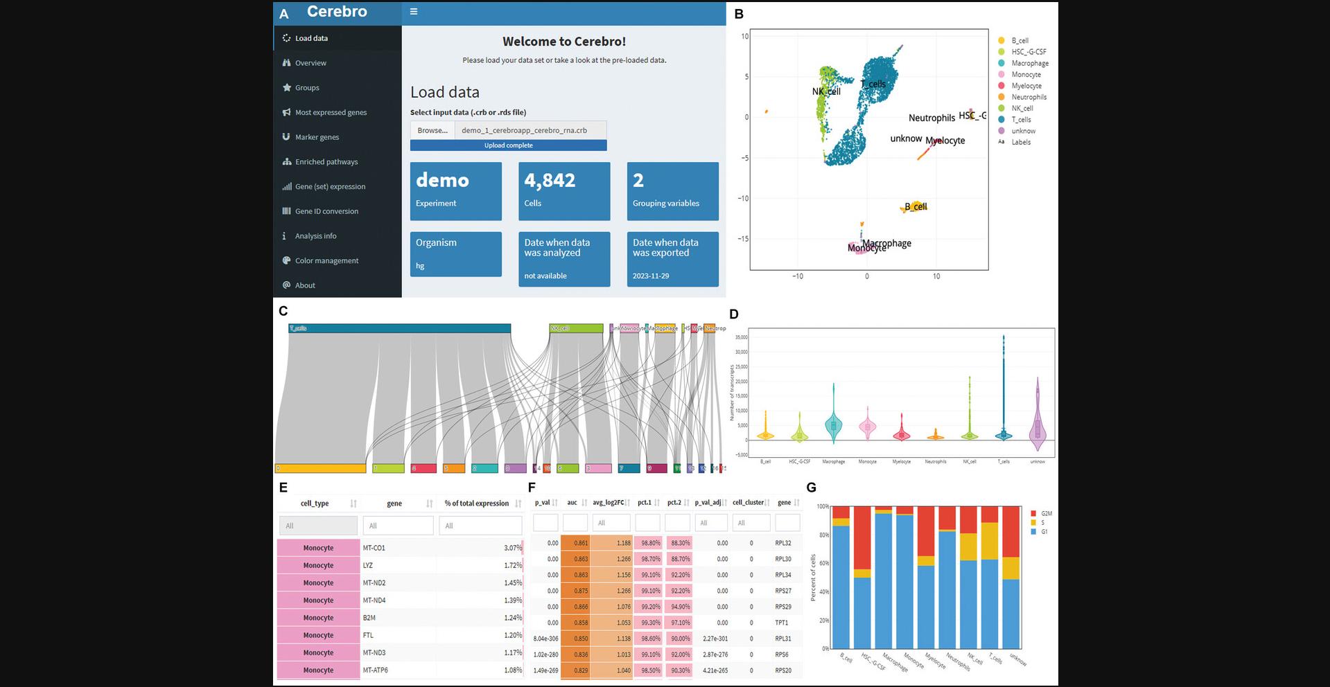
Example plots created with cerebroApp. (A) The Cerebro interface once the RNA data are loaded. (B) Example UMAP plot showing cell type. (C) Sankey plot linking the cell type calls to the Seurat clusters. (D) Violin plot of the transcript counts in each cell type identified. (E) Table of genes ranked by percentage of total expression within one cell group. (F) Table of marker genes highlighted with their p-values and expression levels based on identified clusters. (G) Proportion of cell cycle phases represented in each cell type.

InterCellar

InterCellar is another tool used for the generation of basic plots. In this step, we simply run an R package called InterCellar (Interlandi et al., 2022). This allows us to visualize the results produced by CellphoneDB (results shown in Supporting Information) and CellChat. Like cerebroApp, InterCellar also provides a GUI for data visualization and analysis (Fig. 19). Input files for this package can be generated via Basic Protocol 4, step 8.

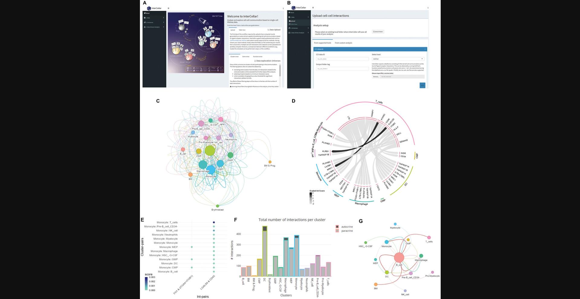
In addition to basic visualization, the InterCellar GUI allows more detailed analysis of cell-cell communication. One can follow the instructions provided by the InterCellar GUI to set up further analysis workflows. We found no issues using this package to further analyze the two human demo samples. However, the current package version (2.0.0) installed via BiocManager::install("InterCellar") or version (2.4.0) installed manually through Package Archives (https://bioconductor.org/packages/release/bioc/html/InterCellar.html) does not work well with the mouse demo data in section Gene-verse. Instead of valid Ensembl and UniProt IDs, the calculation returns “Not-a-Number” values, which introduces errors for further analysis.

# activate interactive user interface.

InterCellar::run_app()

# more information can be found at https://github.com/martaint/InterCellar/

Multiomic analysis with FlowJo

Genomic cytometry allows us to extend the dimensionality of cytometric data using genomic readouts. It is fundamentally no different from approaches such as fluorescent or mass cytometry, and therefore, the data can be visualized using existing flow cytometry analysis packages. By importing the FCS files generated in Basic Protocol 5, it is possible to use programs such as FlowJo to visualize the data. Metrics for visualization are, for example, MT genes, SMK hashtag, RNA counts, RNA features, UMAP dimensions, and pseudotime measures. Importantly, as the data are imported in FCS format, standard data manipulation tools, such as bivariate plotting, overlay, offset and single sample histograms, traditional hierarchal gating, and the potential of back-gating analysis are all available. Figure 20 shows an example of how FlowJo can be used to visualize data.

scRNA-seq analysis with FlowJo. (A) Percentage of MT gene expression in each cell against cell tag numbers. (B) Total number of genes (nFeature_RNA) detected in each cell against cluster numbers. (C) Histogram of cell distribution divided by sample tags. (D) I. UMAP plot showing all cells highlighted by sample tags; II-III. UMAP plots showing tag2 and tag3 cells from demo exp 1, respectively. (E) I-VI. UMAP plots showing cells highlighted by Ab-CD4-CD4, Ab-HLA-DR-CD74, GZMB, Ab-CD19-CD19, Ab-CD56-NCAM1, and Ab-CD8-CD8A, respectively. (F) I. Scatter plot of Ab-CD4-CD4 vs. Ab-CD3-CD3E, and cells are highlighted with Ab-CD8-CD8A expression; II. Scatter dot plots showing CD3D (gene) against Ab-CD3-CD3E, and cells are highlighted with Ab-HLA-DR-CD74. (G) Demo exp 1 CD25+CD62L- population defined by four hierarchal gates from plot I to plot V; VI-IX plots are back gates of the CD25+CD62L- gate.

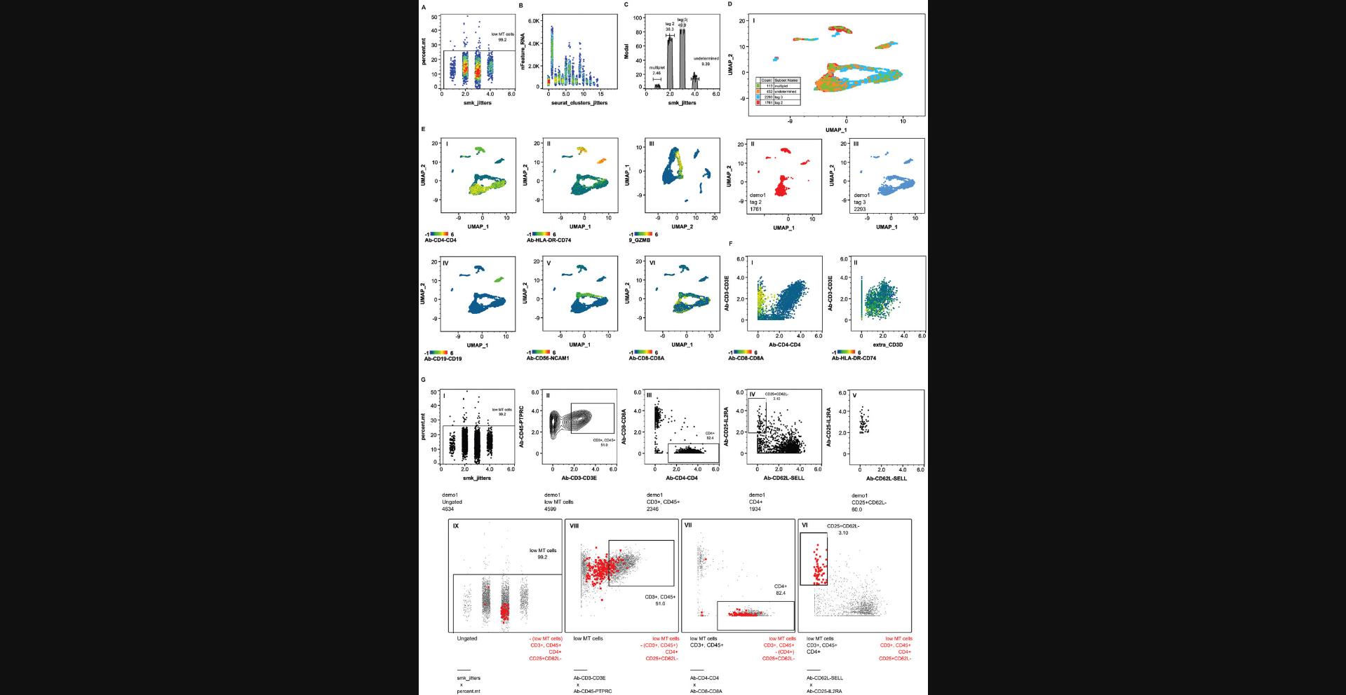
COMMENTARY

Background Information

The workflows demonstrated cover the process from aligning raw reads to a reference genome in SevenBridges to generating a gene expression matrix compatible with the BD Rhapsody chemistry (Basic Protocol 2). Following this, we create Seurat objects from SevenBridges BD Rhapsody pipelines, including targeted sequencing, WTA sequencing, SMK sample tags, and AbSeq (Basic Protocol 3). In addition, we have provided a more detailed pipeline that can be applied to any scRNA-seq data, including 10× Genomics (Basic Protocol 4). Importantly for cytometrists, we have provided a script to convert and export scRNA-seq data into FCS format, which can be viewed and analyzed with standard flow data analysis packages (Basic Protocol 5). Furthermore, we included three different methods/packages (CerebroApp, InterCellar, and FCS software) that minimize R programming while allowing detailed visualization of the generated data (Basic Protocol 6).

Unique to the BD Rhapsody system is the ability to couple cell capture with cell imaging in order to easily assess cell conditions during the cell capture step (Basic Protocol 1). We have found this to be a useful feature when dealing with patient samples, especially when working with cancer cells.

Critical Parameters and Troubleshooting

To prevent data loss, save R data regularly with the following script:

# save R data

save.image(file = paste0(getwd(),"/", "session data.RData"))

SingleR uses curated data as a reference; thus, the input data need to be normalized for cell type predictions to be accurate. In addition, annotation is limited by the reference data in terms of cell type variety. For instance, if the reference dataset does not contain monocytes, true monocytes in the dataset will not be correctly annotated, as there is no reference for this cell type.

Providing correct root cells for monocle3 and slingshot is critical in calculating pseudotime. This protocol uses the results from SingleR to define stem cells. More validations can be done by utilizing other annotation tools or viewing feature gene expression levels.

Infinite or “Not-a-Number” values may exist in pseudotime data or other package outputs, and these values are not handled properly in FlowJo. To bypass this issue, the user should artificially replace these values with constant values so that cells with artificial numbers can be gated out easily for further analysis.

The versions of R, RStudio, and the packages have been provided. It has been seen that the results might be slightly different when different package versions were used. Therefore, to replicate the current results and generate the same figures, we highly recommend that the user force-install the package versions we have used in this study.

The output figures generated have 300-DPI resolution with defined height and width. For generating figures with desired height, width, and DPI, we recommend that users manually adjust the exporting parameters found in func_save_images.

Time Considerations

The time to execute each protocol with a Windows-based 64-bit operating system and x64-based processor with 12th Gen Intel(R) Core(TM) i5-1245U 2.50 GHz, 16.0 GB installed RAM is as follows:

Basic Protocol 1: 19 min and 15 s
Basic Protocol 3: 7 min and 10 s
Basic Protocol 4: 31 min and 20 s
Basic Protocol 5: 45 s
Basic Protocol 6: 9 min and 8 s.

Acknowledgments

We thank the Australian Cancer Research Foundation for supporting this project. We also thank the Medical Research Future Fund through the Emerging Priorities and Consumer Driven Research scheme and the Australian Brain Cancer Mission/National Health & Medical Research Council/Lifting Clinical Trials and Registry Capacity for personnel support.

Open access publishing facilitated by University of New South Wales, as part of the Wiley - University of New South Wales agreement via the Council of Australian University Librarians.

Author Contributions

Wenyan Li : Data curation; formal analysis; investigation; resources; software; writing—original draft; writing—review and editing. Sajad Razavi Bazaz : Software; validation; visualization; writing—original draft; writing—review and editing. Chelsea Mayoh : Methodology; validation; writing—review and editing. Robert Salomon : Conceptualization; formal analysis; funding acquisition; methodology; project administration; supervision; validation; writing—review and editing.

Conflict of Interest

The authors declare no conflicts of interest.

Open Research

Data Availability Statement

The data that support the findings in this article are available in the Supporting Information associated with this article.

Supporting Information

Filename	Description
cpz1963-sup-0001-SuppMat.docx18.7 KB	Instructions to install and use the CellPhoneDB package in a Python programming environment as well as a protocol for running on a mouse dataset.

Please note: The publisher is not responsible for the content or functionality of any supporting information supplied by the authors. Any queries (other than missing content) should be directed to the corresponding author for the article.

Literature Cited

Aran, D., Looney, A. P., Liu, L., Wu, E., Fong, V., Hsu, A., Chak, S., Naikawadi, R. P., Wolters, P. J., Abate, A. R., Butte, A. J., & Bhattacharya, M. (2019). Reference-based analysis of lung single-cell sequencing reveals a transitional profibrotic macrophage. Nature Immunology , 20(2), 163–172. https://doi.org/10.1038/s41590-018-0276-y
Booeshaghi, A. S., Hallgrímsdóttir, I. B., Gálvez-Merchán, Á., & Pachter, L. (2022). Depth normalization for single-cell genomics count data. bioRxiv , 2022.2005.2006.490859. https://doi.org/10.1101/2022.05.06.490859
Briggs, J. A., Weinreb, C., Wagner, D. E., Megason, S., Peshkin, L., Kirschner, M. W., & Klein, A. M. (2018). The dynamics of gene expression in vertebrate embryogenesis at single-cell resolution. Science , 360(6392), eaar5780. https://doi.org/10.1126/science.aar5780
Buenrostro, J. D., Wu, B., Litzenburger, U. M., Ruff, D., Gonzales, M. L., Snyder, M. P., Chang, H. Y., & Greenleaf, W. J. (2015). Single-cell chromatin accessibility reveals principles of regulatory variation. Nature , 523(7561), 486–490. https://doi.org/10.1038/nature14590
Cao, J., Spielmann, M., Qiu, X., Huang, X., Ibrahim, D. M., Hill, A. J., Zhang, F., Mundlos, S., Christiansen, L., Steemers, F. J., Trapnell, C., & Shendure, J. (2019). The single-cell transcriptional landscape of mammalian organogenesis. Nature , 566(7745), 496–502. https://doi.org/10.1038/s41586-019-0969-x
Chen, D., Wang, W., Wu, L., Liang, L., Wang, S., Cheng, Y., Zhang, T., Chai, C., Luo, Q., Sun, C., Zhao, W., Lv, Z., Gao, Y., Wu, X., Sun, N., Zhang, Y., Zhang, J., Chen, Y., Tong, J., … Niu, J. (2022). Single-cell atlas of peripheral blood mononuclear cells from pregnant women. Clinical and Translational Medicine , 12(5), e821. https://doi.org/10.1002/ctm2.821
Collin, J., Queen, R., Zerti, D., Bojic, S., Dorgau, B., Moyse, N., Molina, M. M., Yang, C., Dey, S., Reynolds, G., Hussain, R., Coxhead, J. M., Lisgo, S., Henderson, D., Joseph, A., Rooney, P., Ghosh, S., Clarke, L., Connon, C., … Lako, M. (2021). A single cell atlas of human cornea that defines its development, limbal progenitor cells and their interactions with the immune cells. The Ocular Surface , 21, 279–298. https://doi.org/10.1016/j.jtos.2021.03.010
Efremova, M., Vento-Tormo, M., Teichmann, S. A., & Vento-Tormo, R. (2020). CellPhoneDB: Inferring cell-cell communication from combined expression of multi-subunit ligand-receptor complexes. Nature Protocols , 15(4), 1484–1506. https://doi.org/10.1038/s41596-020-0292-x
Farrell, J. A., Wang, Y., Riesenfeld, S. J., Shekhar, K., Regev, A., & Schier, A. F. (2018). Single-cell reconstruction of developmental trajectories during zebrafish embryogenesis. Science , 360(6392), eaar3131. https://doi.org/10.1126/science.aar3131
Germain, P.-L., Sonrel, A., & Robinson, M. D. (2020). pipeComp, a general framework for the evaluation of computational pipelines, reveals performant single cell RNA-seq preprocessing tools. Genome Biology , 21(1), 227. https://doi.org/10.1186/s13059-020-02136-7
Gierahn, T. M., Wadsworth, M. H., Hughes, T. K., Bryson, B. D., Butler, A., Satija, R., Fortune, S., Love, J. C., & Shalek, A. K. (2017). Seq-Well: Portable, low-cost RNA sequencing of single cells at high throughput. Nature Methods , 14(4), 395–398. https://doi.org/10.1038/nmeth.4179
Gu, Z., Eils, R., & Schlesner, M. (2016). Complex heatmaps reveal patterns and correlations in multidimensional genomic data. Bioinformatics , 32(18), 2847–2849. https://doi.org/10.1093/bioinformatics/btw313
Haghverdi, L., Lun, A. T. L., Morgan, M. D., & Marioni, J. C. (2018). Batch effects in single-cell RNA-sequencing data are corrected by matching mutual nearest neighbors. Nature Biotechnology , 36(5), 421–427. https://doi.org/10.1038/nbt.4091
Hahne, F., LeMeur, N., Brinkman, R. R., Ellis, B., Haaland, P., Sarkar, D., Spidlen, J., Strain, E., & Gentleman, R. (2009). flowCore: A Bioconductor package for high throughput flow cytometry. BMC Bioinformatics , 10, 106. https://doi.org/10.1186/1471-2105-10-106
Hao, Y., Hao, S., Andersen-Nissen, E., Mauck, W. M. 3rd., Zheng, S., Butler, A., Lee, M. J., Wilk, A. J., Darby, C., Zager, M., Hoffman, P., Stoeckius, M., Papalexi, E., Mimitou, E. P., Jain, J., Srivastava, A., Stuart, T., Fleming, L. M., Yeung, B., … Satija, R. (2021). Integrated analysis of multimodal single-cell data. Cell , 184(13), 3573–3587.e3529. https://doi.org/10.1016/j.cell.2021.04.048
Hillje, R., Pelicci, P. G., & Luzi, L. (2020). Cerebro: Interactive visualization of scRNA-seq data. Bioinformatics , 36(7), 2311–2313. https://doi.org/10.1093/bioinformatics/btz877
Hodge, R. D., Bakken, T. E., Miller, J. A., Smith, K. A., Barkan, E. R., Graybuck, L. T., Close, J. L., Long, B., Johansen, N., Penn, O., Yao, Z., Eggermont, J., Höllt, T., Levi, B. P., Shehata, S. I., Aevermann, B., Beller, A., Bertagnolli, D., Brouner, K., … Lein, E. S. (2019). Conserved cell types with divergent features in human versus mouse cortex. Nature , 573(7772), 61–68. https://doi.org/10.1038/s41586-019-1506-7
Hwang, B., Lee, J. H., & Bang, D. (2021). Author correction: Single-cell RNA sequencing technologies and bioinformatics pipelines. Experimental & Molecular Medicine, 53(5), 1005. https://doi.org/10.1038/s12276-021-00615-w
Ilya Korsunsky, A. N., Millard, N., & Raychaudhuri, S. (2022). presto: Fast functions for differential expression using Wilcox and AUC. R package version 1.0.0. https://github.com/immunogenomics/presto/
Interlandi, M., Kerl, K., & Dugas, M. (2022). InterCellar enables interactive analysis and exploration of cell-cell communication in single-cell transcriptomic data. Communications Biology , 5(1), 21. https://doi.org/10.1038/s42003-021-02986-2
Ji, F., & Sadreyev, R. I. (2019). Single-cell RNA-seq: Introduction to bioinformatics analysis. Current Protocols in Molecular Biology , 127(1), e92. https://doi.org/10.1002/cpmb.92
Jin, S., Guerrero-Juarez, C. F., Zhang, L., Chang, I., Ramos, R., Kuan, C. H., Myung, P., Plikus, M. V., & Nie, Q. (2021). Inference and analysis of cell-cell communication using CellChat. Nature Communications , 12(1), 1088. https://doi.org/10.1038/s41467-021-21246-9
Jovic, D., Liang, X., Zeng, H., Lin, L., Xu, F., & Luo, Y. (2022). Single-cell RNA sequencing technologies and applications: A brief overview. Clinical and Translational Medicine , 12(3), e694. https://doi.org/10.1002/ctm2.694
Klein, A. M., Mazutis, L., Akartuna, I., Tallapragada, N., Veres, A., Li, V., Peshkin, L., Weitz, D. A., & Kirschner, M. W. (2015). Droplet barcoding for single-cell transcriptomics applied to embryonic stem cells. Cell , 161(5), 1187–1201. https://doi.org/10.1016/j.cell.2015.04.044
Korsunsky, I., Millard, N., Fan, J., Slowikowski, K., Zhang, F., Wei, K., Baglaenko, Y., Brenner, M., Loh, P. R., & Raychaudhuri, S. (2019). Fast, sensitive and accurate integration of single-cell data with Harmony. Nature Methods , 16(12), 1289–1296. https://doi.org/10.1038/s41592-019-0619-0
Lawlor, N., Nehar-Belaid, D., Grassmann, J. D. S., Stoeckius, M., Smibert, P., Stitzel, M. L., Pascual, V., Banchereau, J., Williams, A., & Ucar, D. (2021). Single cell analysis of blood mononuclear cells stimulated through either LPS or anti-CD3 and anti-CD28. Frontiers in Immunology , 12, 636720. https://doi.org/10.3389/fimmu.2021.636720
Luecken, M. D., & Theis, F. J. (2019). Current best practices in single-cell RNA-seq analysis: A tutorial. Molecular Systems Biology , 15(6), e8746. https://doi.org/10.15252/msb.20188746
Lukowski, S. W., Lo, C. Y., Sharov, A. A., Nguyen, Q., Fang, L., Hung, S. S., Zhu, L., Zhang, T., Grünert, U., Nguyen, T., Senabouth, A., Jabbari, J. S., Welby, E., Sowden, J. C., Waugh, H. S., Mackey, A., Pollock, G., Lamb, T. D., Wang, P.-Y., … Wong, R. C. (2019). A single-cell transcriptome atlas of the adult human retina. The EMBO Journal , 38(18), e100811. https://doi.org/10.15252/embj.2018100811
Macaulay, I. C., Haerty, W., Kumar, P., Li, Y. I., Hu, T. X., Teng, M. J., Goolam, M., Saurat, N., Coupland, P., Shirley, L. M., Smith, M., van der Aa, N., Banerjee, R., Ellis, P. D., Quail, M. A., Swerdlow, H. P., Zernicka-Goetz, M., Livesey, F. J., Ponting, C. P., & Voet, T. (2015). G&T-seq: Parallel sequencing of single-cell genomes and transcriptomes. Nature Methods , 12(6), 519–522. https://doi.org/10.1038/nmeth.3370
Macosko, E. Z., Basu, A., Satija, R., Nemesh, J., Shekhar, K., Goldman, M., Tirosh, I., Bialas, A. R., Kamitaki, N., Martersteck, E. M., Trombetta, J. J., Weitz, D. A., Sanes, J. R., Shalek, A. K., Regev, A., & McCarroll, S. A. (2015). Highly parallel genome-wide expression profiling of individual cells using nanoliter droplets. Cell , 161(5), 1202–1214. https://doi.org/10.1016/j.cell.2015.05.002
McGinnis, C. S., Murrow, L. M., & Gartner, Z. J. (2019). DoubletFinder: Doublet detection in single-cell RNA sequencing data using artificial nearest neighbors. Cell Systems , 8(4), 329–337.e324. https://doi.org/10.1016/j.cels.2019.03.003
Nguyen, Q. H., Pervolarakis, N., Nee, K., & Kessenbrock, K. (2018). Experimental considerations for single-cell RNA sequencing approaches. Frontiers in Cell and Developmental Biology , 6, 108. https://doi.org/10.3389/fcell.2018.00108
Olsen, T. K., & Baryawno, N. (2018). Introduction to single-cell RNA sequencing. Current Protocols in Molecular Biology , 122(1), e57. https://doi.org/10.1002/cpmb.57
Ooms, J. (2022). magick: Advanced graphics and image-processing in R. https://github.com/ropensci/magick; https://docs.ropensci.org/magick/
Paradis, E., & Schliep, K. (2019). ape 5.0: an environment for modern phylogenetics and evolutionary analyses in R. Bioinformatics , 35(3), 526–528, https://doi.org/10.1093/bioinformatics/bty633
Pasquini, G., Rojo Arias, J. E., Schäfer, P., & Busskamp, V. (2021). Automated methods for cell type annotation on scRNA-seq data. Computational and Structural Biotechnology Journal , 19, 961–969. https://doi.org/10.1016/j.csbj.2021.01.015
Pau, G., Fuchs, F., Sklyar, O., Boutros, M., & Huber, W. (2010). EBImage–an R package for image processing with applications to cellular phenotypes. Bioinformatics , 26(7), 979–981. https://doi.org/10.1093/bioinformatics/btq046
Pedersen, T. L. (2020). patchwork: The composer of plots. R package version 1.1.1. https://CRAN.R-project.org/package=patchwork
Pellegrino, M., Sciambi, A., Treusch, S., Durruthy-Durruthy, R., Gokhale, K., Jacob, J., Chen, T. X., Geis, J. A., Oldham, W., Matthews, J., Kantarjian, H., Futreal, P. A., Patel, K., Jones, K. W., Takahashi, K., & Eastburn, D. J. (2018). High-throughput single-cell DNA sequencing of acute myeloid leukemia tumors with droplet microfluidics. Genome Research , 28(9), 1345–1352. https://doi.org/10.1101/gr.232272.117
Peterson, V. M., Zhang, K. X., Kumar, N., Wong, J., Li, L., Wilson, D. C., Moore, R., McClanahan, T. K., Sadekova, S., & Klappenbach, J. A. (2017). Multiplexed quantification of proteins and transcripts in single cells. Nature Biotechnology , 35(10), 936–939. https://doi.org/10.1038/nbt.3973
Qiu, X., Hill, A., Packer, J., Lin, D., Ma, Y. A., & Trapnell, C. (2017). Single-cell mRNA quantification and differential analysis with Census. Nature Methods , 14(3), 309–315. https://doi.org/10.1038/nmeth.4150
Qiu, X., Mao, Q., Tang, Y., Wang, L., Chawla, R., Pliner, H. A., & Trapnell, C. (2017). Reversed graph embedding resolves complex single-cell trajectories. Nature Methods , 14(10), 979–982. https://doi.org/10.1038/nmeth.4402
Rahul Satija, A. B., Hoffman, P., & Stuart, T. (2020). SeuratWrappers: community-provided methods and extensions for the Seurat object. R package version 0.3.0. https://github.com/satijalab/seurat-wrappers
Rotem, A., Ram, O., Shoresh, N., Sperling, R. A., Goren, A., Weitz, D. A., & Bernstein, B. E. (2015). Single-cell ChIP-seq reveals cell subpopulations defined by chromatin state. Nature Biotechnology , 33(11), 1165–1172. https://doi.org/10.1038/nbt.3383
Saelens, W., Cannoodt, R., Todorov, H., & Saeys, Y. (2019). A comparison of single-cell trajectory inference methods. Nature Biotechnology , 37(5), 547–554. https://doi.org/10.1038/s41587-019-0071-9
Salomon, R., Kaczorowski, D., Valdes-Mora, F., Nordon, R. E., Neild, A., Farbehi, N., Bartonicek, N., & Gallego-Ortega, D. (2019). Droplet-based single cell RNAseq tools: A practical guide. Lab on a Chip , 19(10), 1706–1727. https://doi.org/10.1039/c8lc01239c
Salomon, R., Martelotto, L., Valdes-Mora, F., & Gallego-Ortega, D. (2020). Genomic cytometry and new modalities for deep single-cell interrogation. Cytometry Part A , 97(10), 1007–1016. https://doi.org/10.1002/cyto.a.24209
Scherer, S. G. N. R. R. R. A. P. C. M. S. C. (2021). Colorblind-friendly color maps for R. R package version 0.6.2. https://sjmgarnier.github.io/viridis/
Schneider, I., Cepela, J., Shetty, M., Wang, J., Nelson, A. C., Winterhoff, B., & Starr, T. K. (2021). Use of “default” parameter settings when analyzing single cell RNA sequencing data using Seurat: A biologist's perspective. Journal of Translational Genetics and Genomics , 5(1), 37–49. https://doi.org/10.20517/jtgg.2020.48
Shahi, P., Kim, S. C., Haliburton, J. R., Gartner, Z. J., & Abate, A. R. (2017). Abseq: Ultrahigh-throughput single cell protein profiling with droplet microfluidic barcoding. Scientific Reports , 7, 44447. https://doi.org/10.1038/srep44447
Song, H., Weinstein, H. N. W., Allegakoen, P., Wadsworth, M. H., Xie, J., Yang, H., Castro, E. A., Lu, K. L., Stohr, B. A., Feng, F. Y., Carroll, P. R., Wang, B., Cooperberg, M. R., Shalek, A. K., & Huang, F. W. (2022). Single-cell analysis of human primary prostate cancer reveals the heterogeneity of tumor-associated epithelial cell states. Nature Communications , 13(1), 141. https://doi.org/10.1038/s41467-021-27322-4
Speranza, E., Williamson, B. N., Feldmann, F., Sturdevant, G. L., Pérez, L. P.-., Meade-White, K., Smith, B. J., Lovaglio, J., Martens, C., Munster, V. J., Okumura, A., Shaia, C., Feldmann, H., Best, S. M., & Wit, E. D. (2021). Single-cell RNA sequencing reveals SARS-CoV-2 infection dynamics in lungs of African green monkeys. Science Translational Medicine , 13(578), eabe8146. https://doi.org/10.1126/scitranslmed.abe8146
Stoeckius, M., Hafemeister, C., Stephenson, W., Houck-Loomis, B., Chattopadhyay, P. K., Swerdlow, H., Satija, R., & Smibert, P. (2017). Simultaneous epitope and transcriptome measurement in single cells. Nature Methods , 14(9), 865–868. https://doi.org/10.1038/nmeth.4380
Street, K., Risso, D., Fletcher, R. B., Das, D., Ngai, J., Yosef, N., Purdom, E., & Dudoit, S. (2018). Slingshot: Cell lineage and pseudotime inference for single-cell transcriptomics. BMC Genomics , 19(1), 477. https://doi.org/10.1186/s12864-018-4772-0
Trapnell, C., Cacchiarelli, D., Grimsby, J., Pokharel, P., Li, S., Morse, M., Lennon, N. J., Livak, K. J., Mikkelsen, T. S., & Rinn, J. L. (2014). The dynamics and regulators of cell fate decisions are revealed by pseudotemporal ordering of single cells. Nature Biotechnology , 32(4), 381–386. https://doi.org/10.1038/nbt.2859
Valdés-Mora, F., Salomon, R., Gloss, B. S., Law, A. M. K., Venhuizen, J., Castillo, L., Murphy, K. J., Magenau, A., Papanicolaou, M., Rodriguez de la Fuente, L., Roden, D. L., Colino-Sanguino, Y., Kikhtyak, Z., Farbehi, N., Conway, J. R. W., Sikta, N., Oakes, S. R., Cox, T. R., O'Donoghue, S. I., … Gallego-Ortega, D. (2021). Single-cell transcriptomics reveals involution mimicry during the specification of the basal breast cancer subtype. Cell Reports , 35(2), 108945. https://doi.org/10.1016/j.celrep.2021.108945
Wagner, D. E., Weinreb, C., Collins, Z. M., Briggs, J. A., Megason, S. G., & Klein, A. M. (2018). Single-cell mapping of gene expression landscapes and lineage in the zebrafish embryo. Science , 360(6392), 981–987. https://doi.org/10.1126/science.aar4362
Wickham, H., Averick, M., Bryan, J., Chang, W., McGowan, L. D., François, R., Grolemund, G., Hayes, A., Henry, L., Hester, J., Kuhn, M., Pedersen, T. L., Miller, E., Bache, S. M., Müller, K., Ooms, J., Robinson, D., Seidel, D. P., Spinu, V., … Yutani, H. (2019). Welcome to the Tidyverse. Journal of Open Source Software , 4, 1686. https://doi.org/10.21105/joss.01686
Wickham, H., & SpringerLink. (2009). ggplot2: Elegant graphics for data analysis ( 1st ed.). Springer.
Wilson, P. C., Wu, H., Kirita, Y., Uchimura, K., Ledru, N., Rennke, H. G., Welling, P. A., Waikar, S. S., & Humphreys, B. D. (2019). The single-cell transcriptomic landscape of early human diabetic nephropathy. Proceedings of the National Academy of Sciences , 116(39), 19619–19625. https://doi.org/10.1073/pnas.1908706116
Wu, F., Fan, J., He, Y., Xiong, A., Yu, J., Li, Y., Zhang, Y., Zhao, W., Zhou, F., Li, W., Zhang, J., Zhang, X., Qiao, M., Gao, G., Chen, S., Chen, X., Li, X., Hou, L., Wu, C., … Zhou, C. (2021). Single-cell profiling of tumor heterogeneity and the microenvironment in advanced non-small cell lung cancer. Nature Communications , 12(1), 2540. https://doi.org/10.1038/s41467-021-22801-0
Wu, S. Z., Al-Eryani, G., Roden, D. L., Junankar, S., Harvey, K., Andersson, A., Thennavan, A., Wang, C., Torpy, J. R., Bartonicek, N., Wang, T., Larsson, L., Kaczorowski, D., Weisenfeld, N. I., Uytingco, C. R., Chew, J. G., Bent, Z. W., Chan, C. L., Gnanasambandapillai, V., … Swarbrick, A. (2021). A single-cell and spatially resolved atlas of human breast cancers. Nature Genetics , 53(9), 1334–1347. https://doi.org/10.1038/s41588-021-00911-1
Xi, N. M., & Li, J. J. (2021). Benchmarking computational doublet-detection methods for single-cell RNA sequencing data. Cell Systems , 12(2), 176–194.e176. https://doi.org/10.1016/j.cels.2020.11.008
Zhu, L., Yang, P., Zhao, Y., Zhuang, Z., Wang, Z., Song, R., Zhang, J., Liu, C., Gao, Q., Xu, Q., Wei, X., Sun, H. X., Ye, B., Wu, Y., Zhang, N., Lei, G., Yu, L., Yan, J., Diao, G., … Liu, W. J. (2020). Single-cell sequencing of peripheral mononuclear cells reveals distinct immune response landscapes of COVID-19 and influenza patients. Immunity , 53(3), 685–696.e683. https://doi.org/10.1016/j.immuni.2020.07.009

Detect-seq, a chemical labeling and biotin pull-down approach for the unbiased and genome-wide off-target evaluation of programmable cytosine base editors

A systems-level mass spectrometry-based technique for accurate and sensitive quantification of the RNA cap epitranscriptome

References

Abstract
INTRODUCTION
STRATEGIC PLANNING
Basic Protocol 1: IMAGE ANALYSIS
Basic Protocol 2: SEQUENCING QUALITY CONTROL AND GENERATION OF A GENE EXPRESSION MATRIX
Basic Protocol 3: GENE EXPRESSION MATRIX DATA PRE-PROCESSING AND ANALYSIS
Basic Protocol 4: ADVANCED ANALYSIS
Basic Protocol 5: CONVERTING DATA TO FLOW CYTOMETRY STANDARD (FCS) FORMAT
Basic Protocol 6: VISUALIZATION USING GRAPHICAL INTERFACES
COMMENTARY
Open Research
Supporting Information
Literature Cited

Figure 1
BD Rhapsody–based workflows for obtaining high-quality scRNA-seq data. If using solid tissue, digestion must precede sample clean-up prior to loading into the BD Rhapsody capture workflows. Sample clean-up is critical and may involve an optional cell staining and sorting step. Once the cell sample is prepared, it can be loaded into the BD Rhapsody to pair a cell with a polyadenylated paramagnetic bead containing a unique cellular barcode. Following the cell-bead pairing, a sequencing library is created, the library is sequenced, and the data can be analyzed.
Figure 2
Anticipated doublet rates based on cell capture numbers in the BD Rhapsody platform.
Figure 3
This workflow consists of six basic protocols: Basic Protocol 1 - provision of images from the BD Rhapsody™ Scanner produced during cell capture into a manageable format; Basic Protocol 2 - generation of a gene expression matrix from FASTQ files via the SevenBridges online cloud-based computing platform; Basic Protocol 3 - conversion of gene expression matrices from SevenBridges into Seurat objects using R, including the steps to pre-process, perform QC on, and filter the data; Basic Protocol 4 - addition of cell type annotation, cell trajectory analysis, dataset integration, doublet identification, and cell-cell communication into the data analysis; Basic Protocol 5 - conversion of Seurat objects to flow cytometry standard (FCS) format; and Basic Protocol 6 - visualization of data through available GUIs, reducing the need to interface with R.
Figure 4
Folder structure of the working directory required for the protocols to function without modification. The working directory contains four folders: three of them hold the gene expression matrices and corresponding sample tag calls if available, and the other one contains the images and .csv files obtained from the BD Rhapsody™ Scanner. If creating your own script, it must be saved within the working directory.
Figure 5
Overview of Basic Protocol 1. The workflow has three major steps: (1) collect the location and size information for each cell; (2) loop through each image and crop out wells that contain at least one cell; and (3) stitch cropped images as one image or stack images in .gif format.
Figure 6
Representative images produced from Basic Protocol 1 for cells of sizes ranging from 8 to 11 μm and >11 μm, respectively. (A) and (B) Representative array of 64 cells with sizes of 8 to 11 μm imaged by brightfield and fluorescence, respectively. (C) and (D) Representative array of 64 cells with sizes of >11 μm imaged by brightfield and fluorescence, respectively. (E) Histogram of the cell size distribution for all cells. (F) Overlay image of bright-field and fluorescence images for 64 cells.
Figure 7
Inputs and APP settings required for generating the gene expression matrix from BD Rhapsody data in SevenBridges. (A) Files required for the WTA assay. (B) Files required for the targeted panels. (C) APP settings required. The required fields depend on the assays being run, whether sample tags are used, and if subsampling is required. For more details, please consult the manual provided by BD Biosciences.
Figure 8
Outputs generated at the end of a successful pipeline run. Files highlighted with red boxes are the inputs for downstream data analysis in subsequent basic protocols utilizing R.
Figure 9
Cell label filter (left) and cell label second derivative curves (right) for different sample input types. Cell lines will often show a very linear cell label plot and a single sharp drop in the second derivative plot (A), whereas samples like PBMCs (B) or primary patient samples (C) may not be so clear.
Figure 10
QC visualization plots of the data before and after removing cells with high MT content (>50%) and low gene features (cells with less than 200 and 100 RNA molecules, respectively). (A) and (C) Violin plots showing the MT gene percentage in each cluster before and after removing low-quality cells (demo exp 1 and demo exp 2, respectively). (B) and (D) nCount vs. nFeature plots before and after removing low-quality cells (demo exp 1 and demo exp 2, respectively).
Figure 11
UMAP plots generated in Seurat. Cells highlighted by Seurat cluster ID (A) and cells highlighted by sample tags (B). In both panels, the data for demo exp 1 are provided on the left and for demo exp 2 on the right.
Figure 12
Cell annotation using SingleR. (A) and (B) Heatmaps showing cell type prediction scores for the demo exp 1 and demo exp 2 datasets, respectively. (C) UMAP plots with clusters highlighted by cell type.
Figure 13
UMAP plots showing merged datasets before and after batch effect correction using harmony. (A) Merged datasets split by sample, with cell types highlighted. (B) Merged datasets of demo exp 1 and demo exp 2 clustered and highlighted by dataset.
Figure 14
UMAP of demo exp 1 and demo exp 2 highlighted by doublets or singlets identified by DoubletFinder. The left panel shows the doublets for demo exp 1, and the right panel shows doublets for demo exp 2.
Figure 15
Dot plots of demo exp 1 and demo exp 2 showing expression of top marker genes in the cell types identified.
Figure 16
monocle3 analysis of a pooled sample where SampleTag01_hs were non-treated and SampleTag02_hs were activated in the presence of CD3/CD28 for 24 hr. (A) UMAP calculated by monocle3 showing the lineage trajectory and pseudotime. (B) UMAP from Seurat highlighted by pseudotime. (C) Pseudotime comparison between SampleTag01_hs and SampleTag02_hs across all cell types. (D) Scatter plots of gene expression against pseudotime. (E) UMAP from Seurat object subset_demo_seurat_1 first split by sample tag and then highlighted by cell type.
Figure 17
Pseudotime calculation by slingshot. (A) Cell lineages calculated by slingshot displayed on a PCA plot. (B) and (C) Pseudotime comparison between SampleTag01_hs and SampleTag02_hs across all lineage paths and cell types, respectively.
Figure 18
Example plots created with cerebroApp. (A) The Cerebro interface once the RNA data are loaded. (B) Example UMAP plot showing cell type. (C) Sankey plot linking the cell type calls to the Seurat clusters. (D) Violin plot of the transcript counts in each cell type identified. (E) Table of genes ranked by percentage of total expression within one cell group. (F) Table of marker genes highlighted with their p-values and expression levels based on identified clusters. (G) Proportion of cell cycle phases represented in each cell type.
Figure 19
Example plots generated with InterCellar. (A) The InterCellar interface. (B) Analysis setup webpage for InterCellar. (C) Overall cellular communication among clusters. (D) Directed interaction pairs pointing from ligands toward receptors. (E) Selective interaction gene pairs in the network of sender clusters. (F) Total number of interactions per cluster. (G) Cellular communication between B cells and other cell types.
Figure 20
scRNA-seq analysis with FlowJo. (A) Percentage of MT gene expression in each cell against cell tag numbers. (B) Total number of genes (nFeature_RNA) detected in each cell against cluster numbers. (C) Histogram of cell distribution divided by sample tags. (D) I. UMAP plot showing all cells highlighted by sample tags; II-III. UMAP plots showing tag2 and tag3 cells from demo exp 1, respectively. (E) I-VI. UMAP plots showing cells highlighted by Ab-CD4-CD4, Ab-HLA-DR-CD74, GZMB, Ab-CD19-CD19, Ab-CD56-NCAM1, and Ab-CD8-CD8A, respectively. (F) I. Scatter plot of Ab-CD4-CD4 vs. Ab-CD3-CD3E, and cells are highlighted with Ab-CD8-CD8A expression; II. Scatter dot plots showing CD3D (gene) against Ab-CD3-CD3E, and cells are highlighted with Ab-HLA-DR-CD74. (G) Demo exp 1 CD25+CD62L- population defined by four hierarchal gates from plot I to plot V; VI-IX plots are back gates of the CD25+CD62L- gate.

Aran, D., Looney, A. P., Liu, L., Wu, E., Fong, V., Hsu, A., Chak, S., Naikawadi, R. P., Wolters, P. J., Abate, A. R., Butte, A. J., & Bhattacharya, M. (2019). Reference-based analysis of lung single-cell sequencing reveals a transitional profibrotic macrophage. Nature Immunology, 20(2), 163–172. https://doi.org/10.1038/s41590-018-0276-y 10.1038/s41590-018-0276-y CASPubMedWeb of Science®Google Scholar
Booeshaghi, A. S., Hallgrímsdóttir, I. B., Gálvez-Merchán, Á., & Pachter, L. (2022). Depth normalization for single-cell genomics count data. bioRxiv, 2022.2005.2006.490859. https://doi.org/10.1101/2022.05.06.490859 10.1101/2022.05.06.490859 Google Scholar
Briggs, J. A., Weinreb, C., Wagner, D. E., Megason, S., Peshkin, L., Kirschner, M. W., & Klein, A. M. (2018). The dynamics of gene expression in vertebrate embryogenesis at single-cell resolution. Science, 360(6392), eaar5780. https://doi.org/10.1126/science.aar5780 10.1126/science.aar5780 PubMedWeb of Science®Google Scholar
Buenrostro, J. D., Wu, B., Litzenburger, U. M., Ruff, D., Gonzales, M. L., Snyder, M. P., Chang, H. Y., & Greenleaf, W. J. (2015). Single-cell chromatin accessibility reveals principles of regulatory variation. Nature, 523(7561), 486–490. https://doi.org/10.1038/nature14590 10.1038/nature14590 CASPubMedWeb of Science®Google Scholar
Cao, J., Spielmann, M., Qiu, X., Huang, X., Ibrahim, D. M., Hill, A. J., Zhang, F., Mundlos, S., Christiansen, L., Steemers, F. J., Trapnell, C., & Shendure, J. (2019). The single-cell transcriptional landscape of mammalian organogenesis. Nature, 566(7745), 496–502. https://doi.org/10.1038/s41586-019-0969-x 10.1038/s41586-019-0969-x CASADSPubMedWeb of Science®Google Scholar
Chen, D., Wang, W., Wu, L., Liang, L., Wang, S., Cheng, Y., Zhang, T., Chai, C., Luo, Q., Sun, C., Zhao, W., Lv, Z., Gao, Y., Wu, X., Sun, N., Zhang, Y., Zhang, J., Chen, Y., Tong, J., … Niu, J. (2022). Single-cell atlas of peripheral blood mononuclear cells from pregnant women. Clinical and Translational Medicine, 12(5), e821. https://doi.org/10.1002/ctm2.821 10.1002/ctm2.821 CASPubMedWeb of Science®Google Scholar
Collin, J., Queen, R., Zerti, D., Bojic, S., Dorgau, B., Moyse, N., Molina, M. M., Yang, C., Dey, S., Reynolds, G., Hussain, R., Coxhead, J. M., Lisgo, S., Henderson, D., Joseph, A., Rooney, P., Ghosh, S., Clarke, L., Connon, C., … Lako, M. (2021). A single cell atlas of human cornea that defines its development, limbal progenitor cells and their interactions with the immune cells. The Ocular Surface, 21, 279–298. https://doi.org/10.1016/j.jtos.2021.03.010 10.1016/j.jtos.2021.03.010 PubMedWeb of Science®Google Scholar
Efremova, M., Vento-Tormo, M., Teichmann, S. A., & Vento-Tormo, R. (2020). CellPhoneDB: Inferring cell-cell communication from combined expression of multi-subunit ligand-receptor complexes. Nature Protocols, 15(4), 1484–1506. https://doi.org/10.1038/s41596-020-0292-x 10.1038/s41596-020-0292-x CASPubMedWeb of Science®Google Scholar
Farrell, J. A., Wang, Y., Riesenfeld, S. J., Shekhar, K., Regev, A., & Schier, A. F. (2018). Single-cell reconstruction of developmental trajectories during zebrafish embryogenesis. Science, 360(6392), eaar3131. https://doi.org/10.1126/science.aar3131 10.1126/science.aar3131 PubMedWeb of Science®Google Scholar
Germain, P.-L., Sonrel, A., & Robinson, M. D. (2020). pipeComp, a general framework for the evaluation of computational pipelines, reveals performant single cell RNA-seq preprocessing tools. Genome Biology, 21(1), 227. https://doi.org/10.1186/s13059-020-02136-7 10.1186/s13059-020-02136-7 PubMedWeb of Science®Google Scholar
Gierahn, T. M., Wadsworth, M. H., Hughes, T. K., Bryson, B. D., Butler, A., Satija, R., Fortune, S., Love, J. C., & Shalek, A. K. (2017). Seq-Well: Portable, low-cost RNA sequencing of single cells at high throughput. Nature Methods, 14(4), 395–398. https://doi.org/10.1038/nmeth.4179 10.1038/nmeth.4179 CASPubMedWeb of Science®Google Scholar
Gu, Z., Eils, R., & Schlesner, M. (2016). Complex heatmaps reveal patterns and correlations in multidimensional genomic data. Bioinformatics, 32(18), 2847–2849. https://doi.org/10.1093/bioinformatics/btw313 10.1093/bioinformatics/btw313 CASPubMedWeb of Science®Google Scholar
Haghverdi, L., Lun, A. T. L., Morgan, M. D., & Marioni, J. C. (2018). Batch effects in single-cell RNA-sequencing data are corrected by matching mutual nearest neighbors. Nature Biotechnology, 36(5), 421–427. https://doi.org/10.1038/nbt.4091 10.1038/nbt.4091 CASPubMedWeb of Science®Google Scholar
Hahne, F., LeMeur, N., Brinkman, R. R., Ellis, B., Haaland, P., Sarkar, D., Spidlen, J., Strain, E., & Gentleman, R. (2009). flowCore: A Bioconductor package for high throughput flow cytometry. BMC Bioinformatics, 10, 106. https://doi.org/10.1186/1471-2105-10-106 10.1186/1471-2105-10-106 CASPubMedWeb of Science®Google Scholar
Hao, Y., Hao, S., Andersen-Nissen, E., Mauck, W. M. 3rd., Zheng, S., Butler, A., Lee, M. J., Wilk, A. J., Darby, C., Zager, M., Hoffman, P., Stoeckius, M., Papalexi, E., Mimitou, E. P., Jain, J., Srivastava, A., Stuart, T., Fleming, L. M., Yeung, B., … Satija, R. (2021). Integrated analysis of multimodal single-cell data. Cell, 184(13), 3573–3587.e3529. https://doi.org/10.1016/j.cell.2021.04.048 10.1016/j.cell.2021.04.048 CASPubMedWeb of Science®Google Scholar
Hillje, R., Pelicci, P. G., & Luzi, L. (2020). Cerebro: Interactive visualization of scRNA-seq data. Bioinformatics, 36(7), 2311–2313. https://doi.org/10.1093/bioinformatics/btz877 10.1093/bioinformatics/btz877 CASPubMedWeb of Science®Google Scholar
Hodge, R. D., Bakken, T. E., Miller, J. A., Smith, K. A., Barkan, E. R., Graybuck, L. T., Close, J. L., Long, B., Johansen, N., Penn, O., Yao, Z., Eggermont, J., Höllt, T., Levi, B. P., Shehata, S. I., Aevermann, B., Beller, A., Bertagnolli, D., Brouner, K., … Lein, E. S. (2019). Conserved cell types with divergent features in human versus mouse cortex. Nature, 573(7772), 61–68. https://doi.org/10.1038/s41586-019-1506-7 10.1038/s41586-019-1506-7 CASPubMedWeb of Science®Google Scholar
Hwang, B., Lee, J. H., & Bang, D. (2021). Author correction: Single-cell RNA sequencing technologies and bioinformatics pipelines. Experimental & Molecular Medicine, 53(5), 1005. https://doi.org/10.1038/s12276-021-00615-w 10.1038/s12276-021-00615-w CASPubMedWeb of Science®Google Scholar
Ilya Korsunsky, A. N., Millard, N., & Raychaudhuri, S. (2022). presto: Fast functions for differential expression using Wilcox and AUC. R package version 1.0.0. https://github.com/immunogenomics/presto/ Google Scholar
Interlandi, M., Kerl, K., & Dugas, M. (2022). InterCellar enables interactive analysis and exploration of cell-cell communication in single-cell transcriptomic data. Communications Biology, 5(1), 21. https://doi.org/10.1038/s42003-021-02986-2 10.1038/s42003-021-02986-2 CASPubMedWeb of Science®Google Scholar
Ji, F., & Sadreyev, R. I. (2019). Single-cell RNA-seq: Introduction to bioinformatics analysis. Current Protocols in Molecular Biology, 127(1), e92. https://doi.org/10.1002/cpmb.92 10.1002/cpmb.92 PubMedGoogle Scholar
Jin, S., Guerrero-Juarez, C. F., Zhang, L., Chang, I., Ramos, R., Kuan, C. H., Myung, P., Plikus, M. V., & Nie, Q. (2021). Inference and analysis of cell-cell communication using CellChat. Nature Communications, 12(1), 1088. https://doi.org/10.1038/s41467-021-21246-9 10.1038/s41467-021-21246-9 CASPubMedWeb of Science®Google Scholar
Jovic, D., Liang, X., Zeng, H., Lin, L., Xu, F., & Luo, Y. (2022). Single-cell RNA sequencing technologies and applications: A brief overview. Clinical and Translational Medicine, 12(3), e694. https://doi.org/10.1002/ctm2.694 10.1002/ctm2.694 CASPubMedWeb of Science®Google Scholar
Klein, A. M., Mazutis, L., Akartuna, I., Tallapragada, N., Veres, A., Li, V., Peshkin, L., Weitz, D. A., & Kirschner, M. W. (2015). Droplet barcoding for single-cell transcriptomics applied to embryonic stem cells. Cell, 161(5), 1187–1201. https://doi.org/10.1016/j.cell.2015.04.044 10.1016/j.cell.2015.04.044 CASPubMedWeb of Science®Google Scholar
Korsunsky, I., Millard, N., Fan, J., Slowikowski, K., Zhang, F., Wei, K., Baglaenko, Y., Brenner, M., Loh, P. R., & Raychaudhuri, S. (2019). Fast, sensitive and accurate integration of single-cell data with Harmony. Nature Methods, 16(12), 1289–1296. https://doi.org/10.1038/s41592-019-0619-0 10.1038/s41592-019-0619-0 CASPubMedWeb of Science®Google Scholar
Lawlor, N., Nehar-Belaid, D., Grassmann, J. D. S., Stoeckius, M., Smibert, P., Stitzel, M. L., Pascual, V., Banchereau, J., Williams, A., & Ucar, D. (2021). Single cell analysis of blood mononuclear cells stimulated through either LPS or anti-CD3 and anti-CD28. Frontiers in Immunology, 12, 636720. https://doi.org/10.3389/fimmu.2021.636720 10.3389/fimmu.2021.636720 CASPubMedWeb of Science®Google Scholar
Luecken, M. D., & Theis, F. J. (2019). Current best practices in single-cell RNA-seq analysis: A tutorial. Molecular Systems Biology, 15(6), e8746. https://doi.org/10.15252/msb.20188746 10.15252/msb.20188746 PubMedWeb of Science®Google Scholar
Lukowski, S. W., Lo, C. Y., Sharov, A. A., Nguyen, Q., Fang, L., Hung, S. S., Zhu, L., Zhang, T., Grünert, U., Nguyen, T., Senabouth, A., Jabbari, J. S., Welby, E., Sowden, J. C., Waugh, H. S., Mackey, A., Pollock, G., Lamb, T. D., Wang, P.-Y., … Wong, R. C. (2019). A single-cell transcriptome atlas of the adult human retina. The EMBO Journal, 38(18), e100811. https://doi.org/10.15252/embj.2018100811 10.15252/embj.2018100811 PubMedWeb of Science®Google Scholar
Macaulay, I. C., Haerty, W., Kumar, P., Li, Y. I., Hu, T. X., Teng, M. J., Goolam, M., Saurat, N., Coupland, P., Shirley, L. M., Smith, M., van der Aa, N., Banerjee, R., Ellis, P. D., Quail, M. A., Swerdlow, H. P., Zernicka-Goetz, M., Livesey, F. J., Ponting, C. P., & Voet, T. (2015). G&T-seq: Parallel sequencing of single-cell genomes and transcriptomes. Nature Methods, 12(6), 519–522. https://doi.org/10.1038/nmeth.3370 10.1038/nmeth.3370 CASPubMedWeb of Science®Google Scholar
Macosko, E. Z., Basu, A., Satija, R., Nemesh, J., Shekhar, K., Goldman, M., Tirosh, I., Bialas, A. R., Kamitaki, N., Martersteck, E. M., Trombetta, J. J., Weitz, D. A., Sanes, J. R., Shalek, A. K., Regev, A., & McCarroll, S. A. (2015). Highly parallel genome-wide expression profiling of individual cells using nanoliter droplets. Cell, 161(5), 1202–1214. https://doi.org/10.1016/j.cell.2015.05.002 10.1016/j.cell.2015.05.002 CASPubMedWeb of Science®Google Scholar
McGinnis, C. S., Murrow, L. M., & Gartner, Z. J. (2019). DoubletFinder: Doublet detection in single-cell RNA sequencing data using artificial nearest neighbors. Cell Systems, 8(4), 329–337.e324. https://doi.org/10.1016/j.cels.2019.03.003 10.1016/j.cels.2019.03.003 CASPubMedWeb of Science®Google Scholar
Nguyen, Q. H., Pervolarakis, N., Nee, K., & Kessenbrock, K. (2018). Experimental considerations for single-cell RNA sequencing approaches. Frontiers in Cell and Developmental Biology, 6, 108. https://doi.org/10.3389/fcell.2018.00108 10.3389/fcell.2018.00108 PubMedWeb of Science®Google Scholar
Olsen, T. K., & Baryawno, N. (2018). Introduction to single-cell RNA sequencing. Current Protocols in Molecular Biology, 122(1), e57. https://doi.org/10.1002/cpmb.57 10.1002/cpmb.57 PubMedGoogle Scholar
Ooms, J. (2022). magick: Advanced graphics and image-processing in R. https://github.com/ropensci/magick; https://docs.ropensci.org/magick/ Google Scholar
Paradis, E., & Schliep, K. (2019). ape 5.0: an environment for modern phylogenetics and evolutionary analyses in R. Bioinformatics, 35(3), 526–528, https://doi.org/10.1093/bioinformatics/bty633 10.1093/bioinformatics/bty633 CASPubMedWeb of Science®Google Scholar
Pasquini, G., Rojo Arias, J. E., Schäfer, P., & Busskamp, V. (2021). Automated methods for cell type annotation on scRNA-seq data. Computational and Structural Biotechnology Journal, 19, 961–969. https://doi.org/10.1016/j.csbj.2021.01.015 10.1016/j.csbj.2021.01.015 CASPubMedWeb of Science®Google Scholar
Pau, G., Fuchs, F., Sklyar, O., Boutros, M., & Huber, W. (2010). EBImage–an R package for image processing with applications to cellular phenotypes. Bioinformatics, 26(7), 979–981. https://doi.org/10.1093/bioinformatics/btq046 10.1093/bioinformatics/btq046 CASPubMedWeb of Science®Google Scholar
Pedersen, T. L. (2020). patchwork: The composer of plots. R package version 1.1.1. https://CRAN.R-project.org/package=patchwork Google Scholar
Pellegrino, M., Sciambi, A., Treusch, S., Durruthy-Durruthy, R., Gokhale, K., Jacob, J., Chen, T. X., Geis, J. A., Oldham, W., Matthews, J., Kantarjian, H., Futreal, P. A., Patel, K., Jones, K. W., Takahashi, K., & Eastburn, D. J. (2018). High-throughput single-cell DNA sequencing of acute myeloid leukemia tumors with droplet microfluidics. Genome Research, 28(9), 1345–1352. https://doi.org/10.1101/gr.232272.117 10.1101/gr.232272.117 CASPubMedWeb of Science®Google Scholar
Peterson, V. M., Zhang, K. X., Kumar, N., Wong, J., Li, L., Wilson, D. C., Moore, R., McClanahan, T. K., Sadekova, S., & Klappenbach, J. A. (2017). Multiplexed quantification of proteins and transcripts in single cells. Nature Biotechnology, 35(10), 936–939. https://doi.org/10.1038/nbt.3973 10.1038/nbt.3973 CASPubMedWeb of Science®Google Scholar
Qiu, X., Hill, A., Packer, J., Lin, D., Ma, Y. A., & Trapnell, C. (2017). Single-cell mRNA quantification and differential analysis with Census. Nature Methods, 14(3), 309–315. https://doi.org/10.1038/nmeth.4150 10.1038/nmeth.4150 CASPubMedWeb of Science®Google Scholar
Qiu, X., Mao, Q., Tang, Y., Wang, L., Chawla, R., Pliner, H. A., & Trapnell, C. (2017). Reversed graph embedding resolves complex single-cell trajectories. Nature Methods, 14(10), 979–982. https://doi.org/10.1038/nmeth.4402 10.1038/nmeth.4402 CASPubMedWeb of Science®Google Scholar
Rahul Satija, A. B., Hoffman, P., & Stuart, T. (2020). SeuratWrappers: community-provided methods and extensions for the Seurat object. R package version 0.3.0. https://github.com/satijalab/seurat-wrappers Google Scholar
Rotem, A., Ram, O., Shoresh, N., Sperling, R. A., Goren, A., Weitz, D. A., & Bernstein, B. E. (2015). Single-cell ChIP-seq reveals cell subpopulations defined by chromatin state. Nature Biotechnology, 33(11), 1165–1172. https://doi.org/10.1038/nbt.3383 10.1038/nbt.3383 CASPubMedWeb of Science®Google Scholar
Saelens, W., Cannoodt, R., Todorov, H., & Saeys, Y. (2019). A comparison of single-cell trajectory inference methods. Nature Biotechnology, 37(5), 547–554. https://doi.org/10.1038/s41587-019-0071-9 10.1038/s41587-019-0071-9 CASPubMedWeb of Science®Google Scholar
Salomon, R., Kaczorowski, D., Valdes-Mora, F., Nordon, R. E., Neild, A., Farbehi, N., Bartonicek, N., & Gallego-Ortega, D. (2019). Droplet-based single cell RNAseq tools: A practical guide. Lab on a Chip, 19(10), 1706–1727. https://doi.org/10.1039/c8lc01239c 10.1039/C8LC01239C CASPubMedWeb of Science®Google Scholar
Salomon, R., Martelotto, L., Valdes-Mora, F., & Gallego-Ortega, D. (2020). Genomic cytometry and new modalities for deep single-cell interrogation. Cytometry Part A, 97(10), 1007–1016. https://doi.org/10.1002/cyto.a.24209 10.1002/cyto.a.24209 PubMedWeb of Science®Google Scholar
Scherer, S. G. N. R. R. R. A. P. C. M. S. C. (2021). Colorblind-friendly color maps for R. R package version 0.6.2. https://sjmgarnier.github.io/viridis/ Google Scholar
Schneider, I., Cepela, J., Shetty, M., Wang, J., Nelson, A. C., Winterhoff, B., & Starr, T. K. (2021). Use of “default” parameter settings when analyzing single cell RNA sequencing data using Seurat: A biologist's perspective. Journal of Translational Genetics and Genomics, 5(1), 37–49. https://doi.org/10.20517/jtgg.2020.48 10.20517/jtgg.2020.48 CASGoogle Scholar
Shahi, P., Kim, S. C., Haliburton, J. R., Gartner, Z. J., & Abate, A. R. (2017). Abseq: Ultrahigh-throughput single cell protein profiling with droplet microfluidic barcoding. Scientific Reports, 7, 44447. https://doi.org/10.1038/srep44447 10.1038/srep44447 CASPubMedWeb of Science®Google Scholar
Song, H., Weinstein, H. N. W., Allegakoen, P., Wadsworth, M. H., Xie, J., Yang, H., Castro, E. A., Lu, K. L., Stohr, B. A., Feng, F. Y., Carroll, P. R., Wang, B., Cooperberg, M. R., Shalek, A. K., & Huang, F. W. (2022). Single-cell analysis of human primary prostate cancer reveals the heterogeneity of tumor-associated epithelial cell states. Nature Communications, 13(1), 141. https://doi.org/10.1038/s41467-021-27322-4 10.1038/s41467-021-27322-4 CASPubMedWeb of Science®Google Scholar
Speranza, E., Williamson, B. N., Feldmann, F., Sturdevant, G. L., Pérez, L. P.-., Meade-White, K., Smith, B. J., Lovaglio, J., Martens, C., Munster, V. J., Okumura, A., Shaia, C., Feldmann, H., Best, S. M., & Wit, E. D. (2021). Single-cell RNA sequencing reveals SARS-CoV-2 infection dynamics in lungs of African green monkeys. Science Translational Medicine, 13(578), eabe8146. https://doi.org/10.1126/scitranslmed.abe8146 10.1126/scitranslmed.abe8146 CASPubMedWeb of Science®Google Scholar
Stoeckius, M., Hafemeister, C., Stephenson, W., Houck-Loomis, B., Chattopadhyay, P. K., Swerdlow, H., Satija, R., & Smibert, P. (2017). Simultaneous epitope and transcriptome measurement in single cells. Nature Methods, 14(9), 865–868. https://doi.org/10.1038/nmeth.4380 10.1038/nmeth.4380 CASPubMedWeb of Science®Google Scholar
Street, K., Risso, D., Fletcher, R. B., Das, D., Ngai, J., Yosef, N., Purdom, E., & Dudoit, S. (2018). Slingshot: Cell lineage and pseudotime inference for single-cell transcriptomics. BMC Genomics, 19(1), 477. https://doi.org/10.1186/s12864-018-4772-0 10.1186/s12864-018-4772-0 PubMedWeb of Science®Google Scholar
Trapnell, C., Cacchiarelli, D., Grimsby, J., Pokharel, P., Li, S., Morse, M., Lennon, N. J., Livak, K. J., Mikkelsen, T. S., & Rinn, J. L. (2014). The dynamics and regulators of cell fate decisions are revealed by pseudotemporal ordering of single cells. Nature Biotechnology, 32(4), 381–386. https://doi.org/10.1038/nbt.2859 10.1038/nbt.2859 CASPubMedWeb of Science®Google Scholar
Valdés-Mora, F., Salomon, R., Gloss, B. S., Law, A. M. K., Venhuizen, J., Castillo, L., Murphy, K. J., Magenau, A., Papanicolaou, M., Rodriguez de la Fuente, L., Roden, D. L., Colino-Sanguino, Y., Kikhtyak, Z., Farbehi, N., Conway, J. R. W., Sikta, N., Oakes, S. R., Cox, T. R., O'Donoghue, S. I., … Gallego-Ortega, D. (2021). Single-cell transcriptomics reveals involution mimicry during the specification of the basal breast cancer subtype. Cell Reports, 35(2), 108945. https://doi.org/10.1016/j.celrep.2021.108945 10.1016/j.celrep.2021.108945 CASPubMedWeb of Science®Google Scholar
Wagner, D. E., Weinreb, C., Collins, Z. M., Briggs, J. A., Megason, S. G., & Klein, A. M. (2018). Single-cell mapping of gene expression landscapes and lineage in the zebrafish embryo. Science, 360(6392), 981–987. https://doi.org/10.1126/science.aar4362 10.1126/science.aar4362 CASPubMedWeb of Science®Google Scholar
Wickham, H., Averick, M., Bryan, J., Chang, W., McGowan, L. D., François, R., Grolemund, G., Hayes, A., Henry, L., Hester, J., Kuhn, M., Pedersen, T. L., Miller, E., Bache, S. M., Müller, K., Ooms, J., Robinson, D., Seidel, D. P., Spinu, V., … Yutani, H. (2019). Welcome to the Tidyverse. Journal of Open Source Software, 4, 1686. https://doi.org/10.21105/joss.01686 10.21105/joss.01686 Google Scholar
Wickham, H., & SpringerLink. (2009). ggplot2: Elegant graphics for data analysis ( 1st ed.). Springer. 10.1007/978-0-387-98141-3 Web of Science®Google Scholar
Wilson, P. C., Wu, H., Kirita, Y., Uchimura, K., Ledru, N., Rennke, H. G., Welling, P. A., Waikar, S. S., & Humphreys, B. D. (2019). The single-cell transcriptomic landscape of early human diabetic nephropathy. Proceedings of the National Academy of Sciences, 116(39), 19619–19625. https://doi.org/10.1073/pnas.1908706116 10.1073/pnas.1908706116 CASPubMedWeb of Science®Google Scholar
Wu, F., Fan, J., He, Y., Xiong, A., Yu, J., Li, Y., Zhang, Y., Zhao, W., Zhou, F., Li, W., Zhang, J., Zhang, X., Qiao, M., Gao, G., Chen, S., Chen, X., Li, X., Hou, L., Wu, C., … Zhou, C. (2021). Single-cell profiling of tumor heterogeneity and the microenvironment in advanced non-small cell lung cancer. Nature Communications, 12(1), 2540. https://doi.org/10.1038/s41467-021-22801-0 10.1038/s41467-021-22801-0 CASPubMedWeb of Science®Google Scholar
Wu, S. Z., Al-Eryani, G., Roden, D. L., Junankar, S., Harvey, K., Andersson, A., Thennavan, A., Wang, C., Torpy, J. R., Bartonicek, N., Wang, T., Larsson, L., Kaczorowski, D., Weisenfeld, N. I., Uytingco, C. R., Chew, J. G., Bent, Z. W., Chan, C. L., Gnanasambandapillai, V., … Swarbrick, A. (2021). A single-cell and spatially resolved atlas of human breast cancers. Nature Genetics, 53(9), 1334–1347. https://doi.org/10.1038/s41588-021-00911-1 10.1038/s41588-021-00911-1 CASPubMedWeb of Science®Google Scholar
Xi, N. M., & Li, J. J. (2021). Benchmarking computational doublet-detection methods for single-cell RNA sequencing data. Cell Systems, 12(2), 176–194.e176. https://doi.org/10.1016/j.cels.2020.11.008 10.1016/j.cels.2020.11.008 CASPubMedWeb of Science®Google Scholar
Zhu, L., Yang, P., Zhao, Y., Zhuang, Z., Wang, Z., Song, R., Zhang, J., Liu, C., Gao, Q., Xu, Q., Wei, X., Sun, H. X., Ye, B., Wu, Y., Zhang, N., Lei, G., Yu, L., Yan, J., Diao, G., … Liu, W. J. (2020). Single-cell sequencing of peripheral mononuclear cells reveals distinct immune response landscapes of COVID-19 and influenza patients. Immunity, 53(3), 685–696.e683. https://doi.org/10.1016/j.immuni.2020.07.009 10.1016/j.immuni.2020.07.009 CASPubMedWeb of Science®Google Scholar

Analytical Workflows for Single-Cell Multiomic Data Using the BD Rhapsody Platform

Abstract

INTRODUCTION

STRATEGIC PLANNING

Considerations before Initiating the Data Analysis

Basic Protocol 1: IMAGE ANALYSIS

Relevance

Current Limitations

Anticipated Results

Necessary Resources

Basic Protocol 2: SEQUENCING QUALITY CONTROL AND GENERATION OF A GENE EXPRESSION MATRIX

Relevance

Current Limitations

Necessary Resources

Data loading and FASTQ processing to create a gene expression matrix

Pipeline output from the SevenBridges platform

Basic Protocol 3: GENE EXPRESSION MATRIX DATA PRE-PROCESSING AND ANALYSIS

Relevance

Current Limitations

Necessary Resources

Basic Protocol 4: ADVANCED ANALYSIS

Relevance

Current Limitations

Necessary Resources

Basic Protocol 5: CONVERTING DATA TO FLOW CYTOMETRY STANDARD (FCS) FORMAT

Relevance

Current Limitations

Necessary Resources

Basic Protocol 6: VISUALIZATION USING GRAPHICAL INTERFACES

Relevance

Current Limitations

Necessary Resources

cerebroApp

InterCellar

Multiomic analysis with FlowJo

COMMENTARY

Background Information

Critical Parameters and Troubleshooting

Time Considerations

Acknowledgments

Author Contributions

Conflict of Interest

Open Research

Data Availability Statement

Supporting Information

Literature Cited

推荐阅读