An experimental approach on dynamic Occlusal Fingerprint Analysis to simulate use-wear development and localisation on stone tools

Experimental tools

Two blades with a natural sample morphology are knapped for the experiment.

2blades

Raw material

Baltic flint; Southern Sweden (secondary deposit) with the following coordinates:

55.945852 N, 12.767851 E

Note: This raw material is used for all samples.

Knapped tool samples

The raw material is knapped into blades. Both blades are retouched laterally.

a) Tool sample FLT13-1 (knapped by Olaf Jöris) is retouched with direct impacts from a hard hammer (pebble) and has the following dimensions:

83.4 mm length

27.3 mm width

6.3 mm thickness

b) Tool sample FLT13-12 (knapped by Frank Moseler) is retouched with direct impacts from a hard hammer (pebble) and has the following dimensions:

71.9 mm length

21.5 mm width

8.4 mm thickness

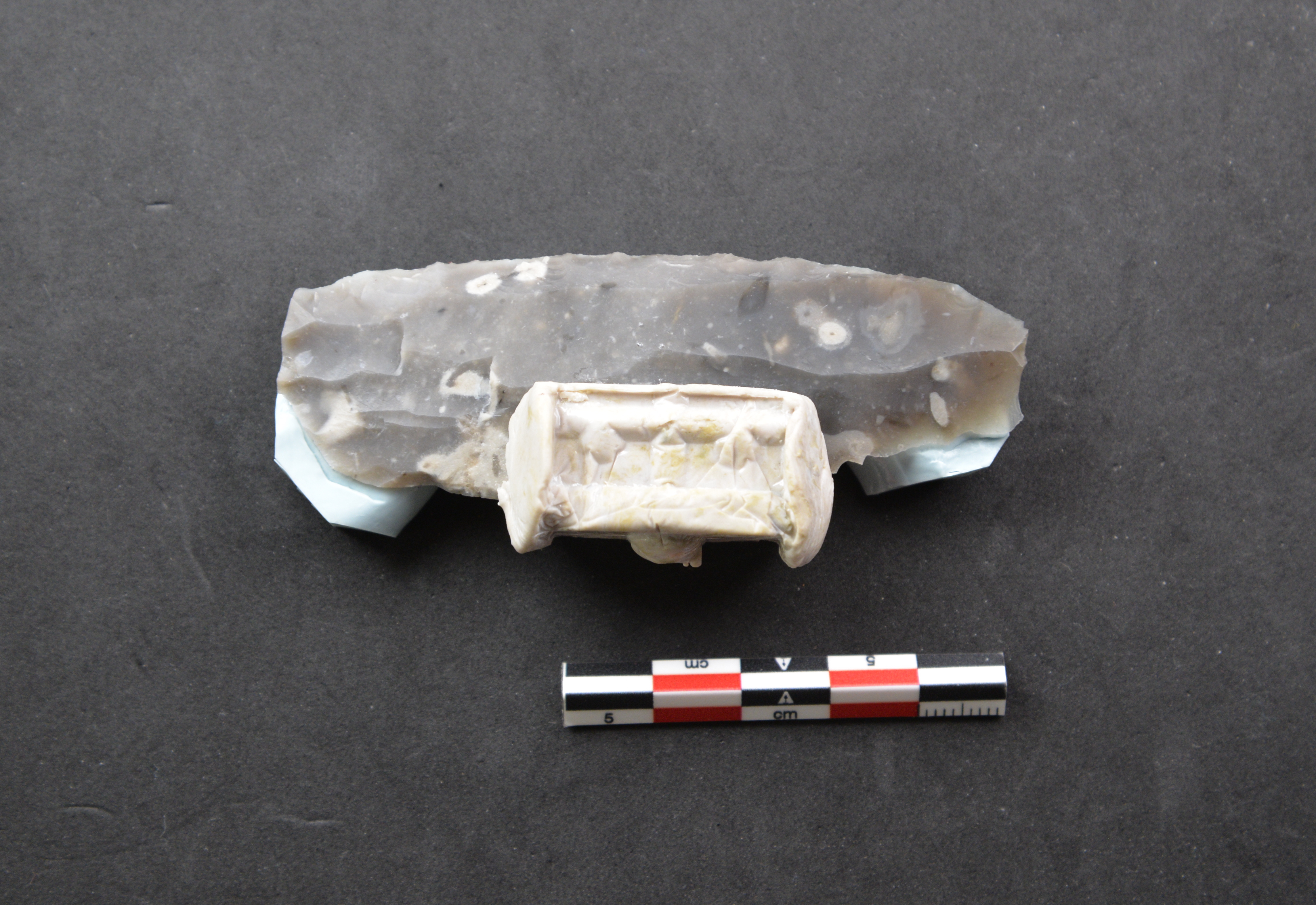
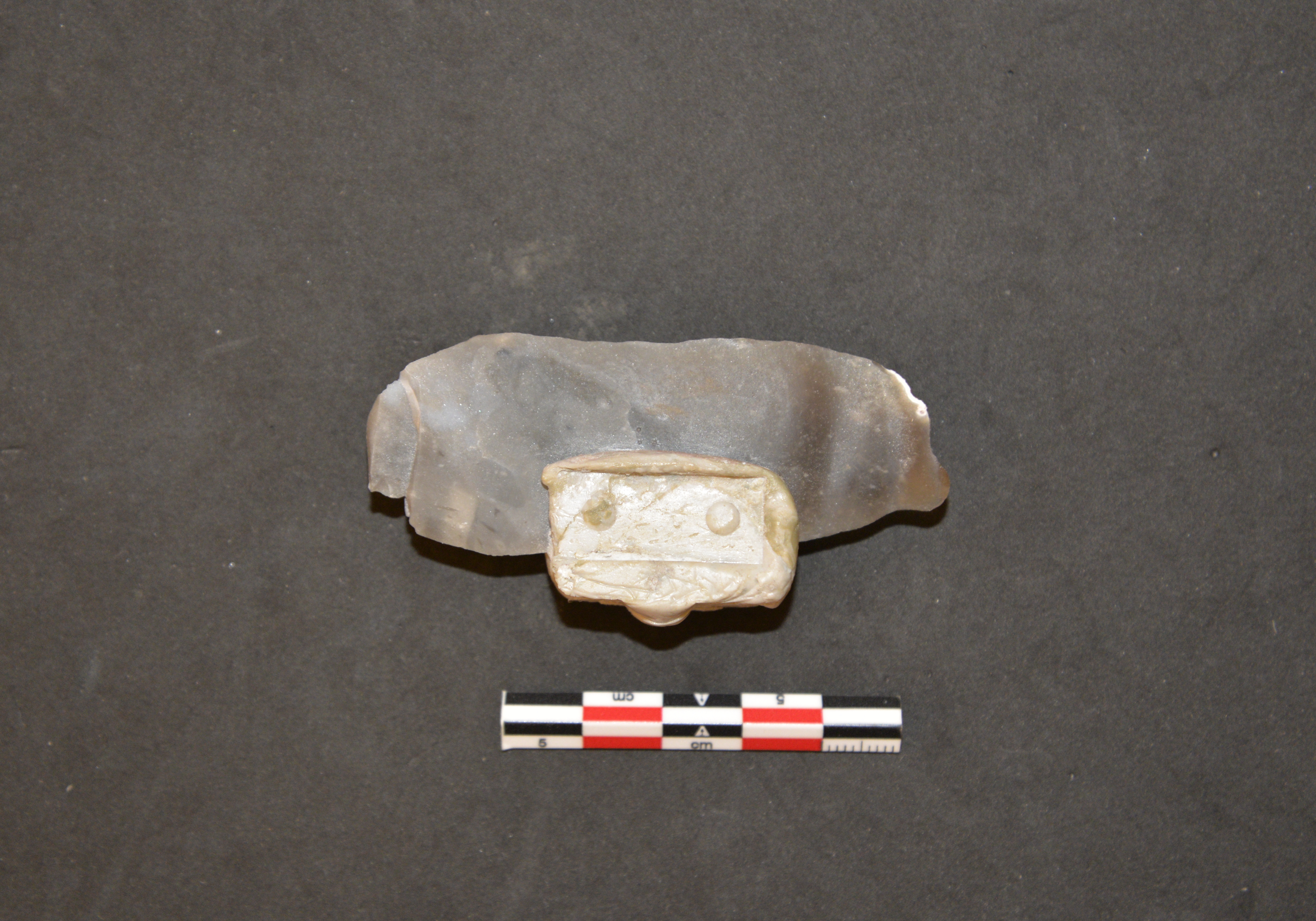
Sample clamps

Sample clamps are prepared for cutting cycles with the SMARTTESTER® (step #9).

a) epoxy paste is cut15 mm

b) mass is kneaded

c) plastic foil is spanned in the clamp

d) the mass is placed in the sample holder from the SMARTTESTER®

e) the blade is added and the screw of the sample holder (SMARTTESTER®) is tightened

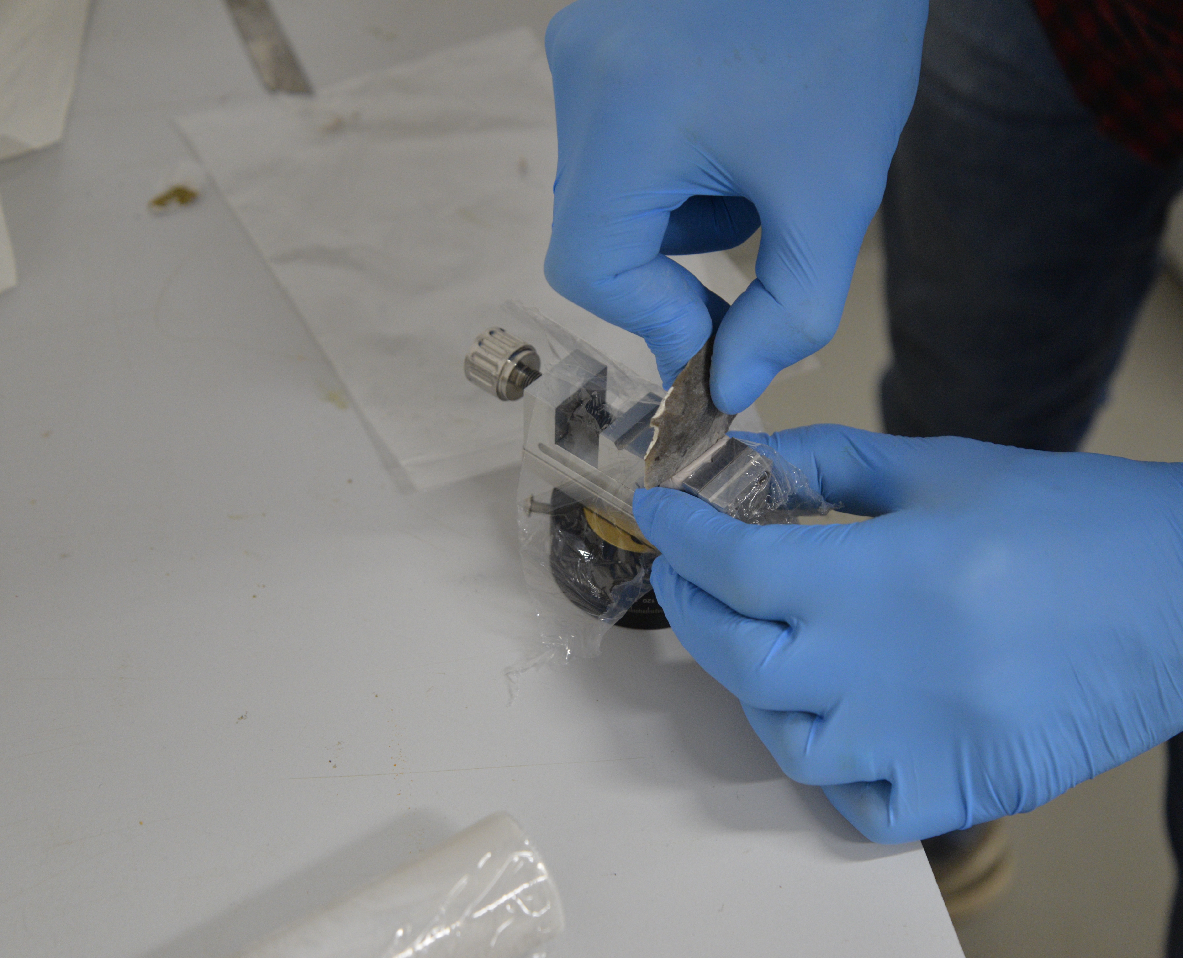
f) the holder is left to set 12h 0m 0s

Sample supports

Sample supports are made for holding the knapped samples during documentation. The following silicone components are mixed:

20g

20g

The silicone sample holder is left to set 0h 25m 0s at 25°C

Standardised tool samples

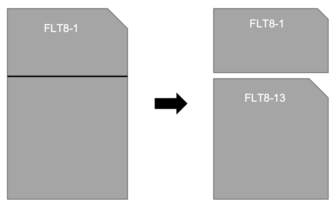
Two experimental standard saw-cut tool samples with a 45° edge angle are produced for the experiment.

2x 45°

Flakes

a) Tool sample FLT8-1 and its acquired experimental data was adopted from a previous study from Lisa Schunk et al. 2021:

Tool sample FLT8-1 has the following dimensions:

24.6 mm length

46.6 mm width

10.8 mm thickness

b) Tool sample FLT8-13 is produced by sawing off the base of sample FLT8-1 with a diamond saw. Then, an edge angle of 45° is cut using the diamond saw.

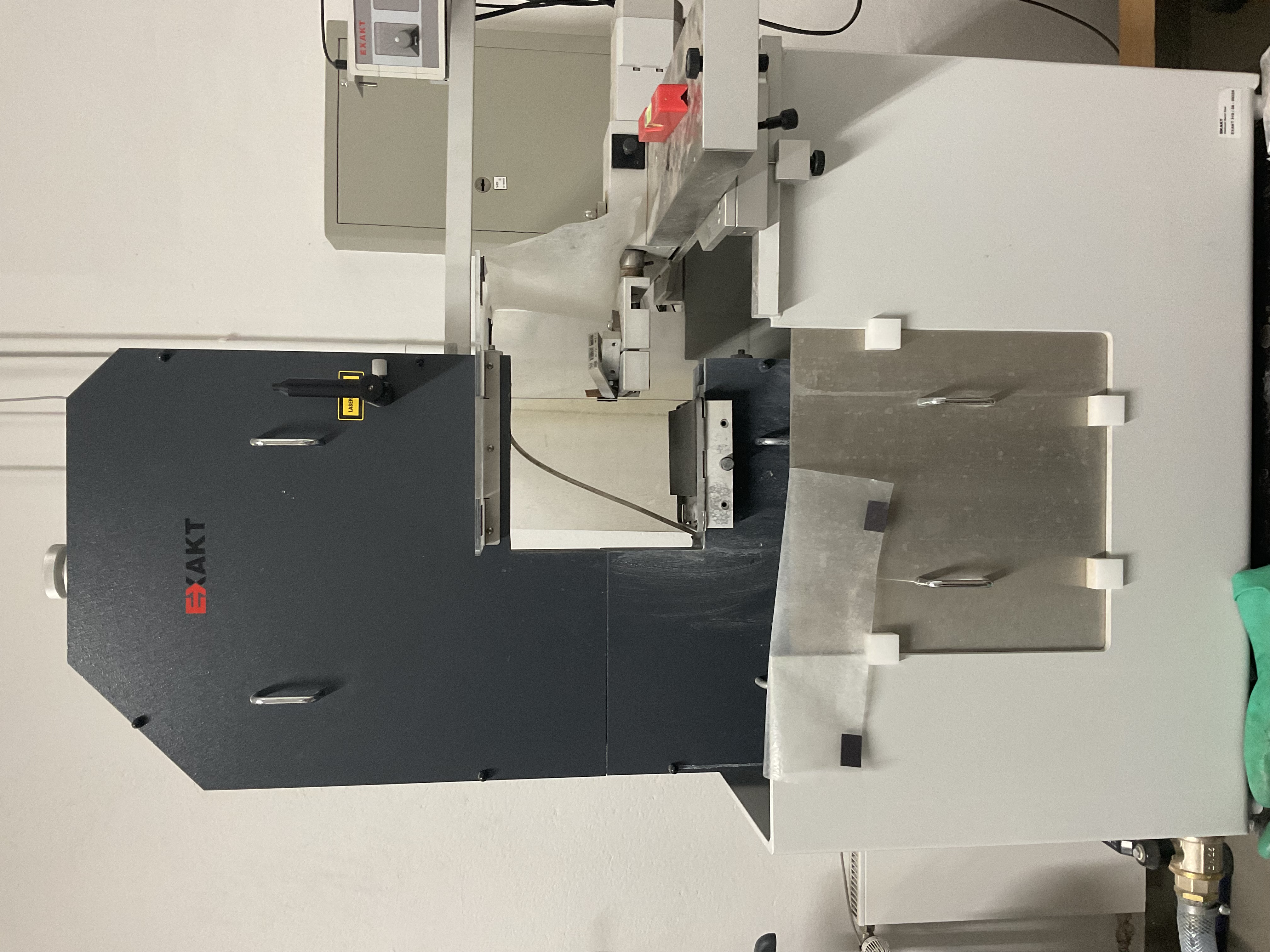
Equipment

Value	Label
310 CP	NAME
Diamond band saw	TYPE
Exact	BRAND
-	SKU

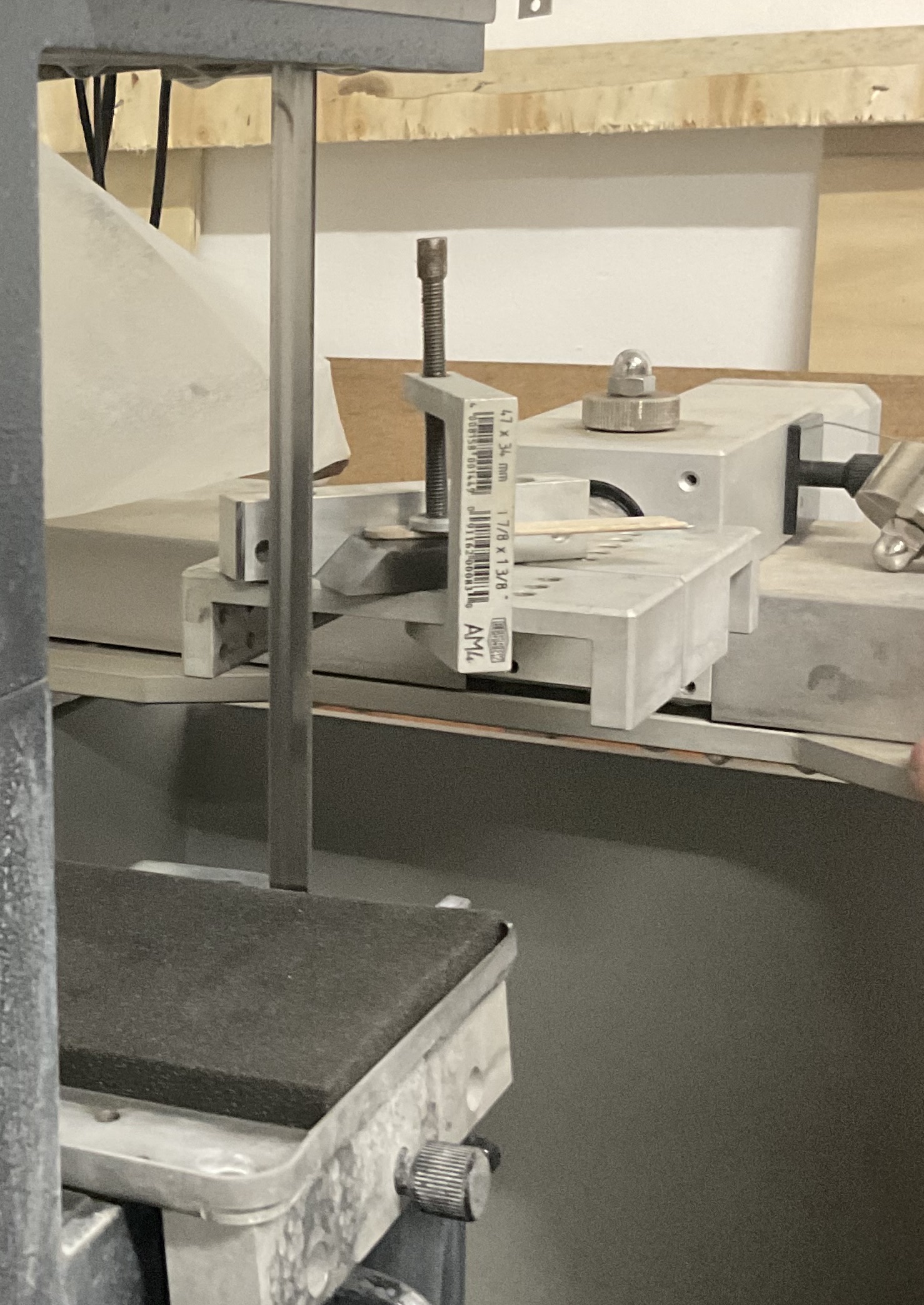
b) To avoid catastrophic breakage of the edge during experiments, the leading edge of tool sample FLT8-13 is chamfered at 45° . The same protocol was also applied to FLT8-1 in Schunk et al. 2021.

Equipment

Value	Label
310 CP	NAME
Diamond band saw	TYPE
Exact	BRAND
-	SKU

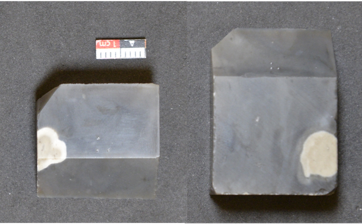
Tool sample FLT8-13 has the following dimensions:

24.4 mm length

24.5 mm width

8.4 mm thickness

Cleaning

After sample preparation, the saw-cut tool samples are cleaned to remove any residues that accumulated during preparation:

1. Tool samples are rinsed with tap water.

2. Tool samples are individually packed in plastic bags filled with demineralised water and a surfactant:

100mL

1Mass

3. The bags are suspended in a preheated ultrasonic bath for 5 minutes at 100 KHz.

Equipment

Value	Label
Heated ultrasonic bath	NAME
Sonorex Digitec DT255H	BRAND
62083	SKU
https://ultraschall-welt.de/ultraschallreiniger/serien/bandelin-geraete/269/bandelin-sonorex-digitec-dt-255-h-5-5?c=0	LINK

0h 5m 0s

40°C

4. Lastly, the tool samples are rinsed in their plastic bags with purified water.

The cleaning protocol for the knapped tool samples was simpler as there are fewer residues produced during their preparation. The edge of each blade was treated with acetone applied with cotton swabs.

Fibers from the swabs were removed with an air compressor.

Equipment

Value	Label
480W Silent Flüsterkompressor Druckluftkompressor	NAME
Modell: 1-480-9	TYPE
IMPLOTEX	BRAND
Artikelnummer NEW-325	SKU
https://www.implotex.de/	LINK

Natural contact material

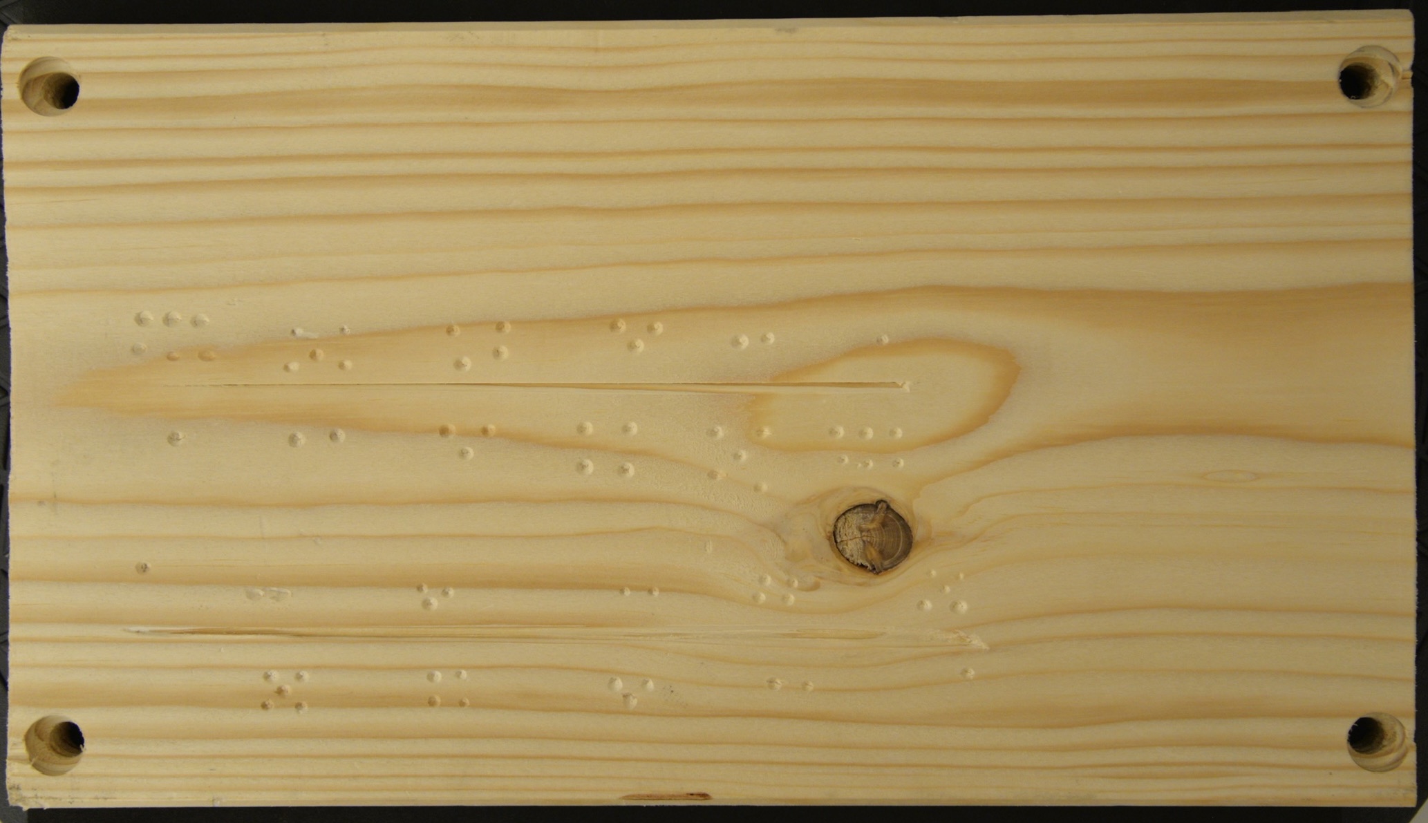
A slab of pine wood ( Pinus sylvestris ) with the following dimensions is used as a contact material:

300 mm length

165 mm width

20 mm thickness

Pine wood is used as a contact material for the following tool samples:

1. Saw-cut flake tool FLT8-13
2. Knapped blade tool FLT13-12

After the first set of experiments, circular marks along the cut groove are added with a center punch to aid in 3D contour matching (step #7.2 and #9.5).

Standardised synthetic contact material

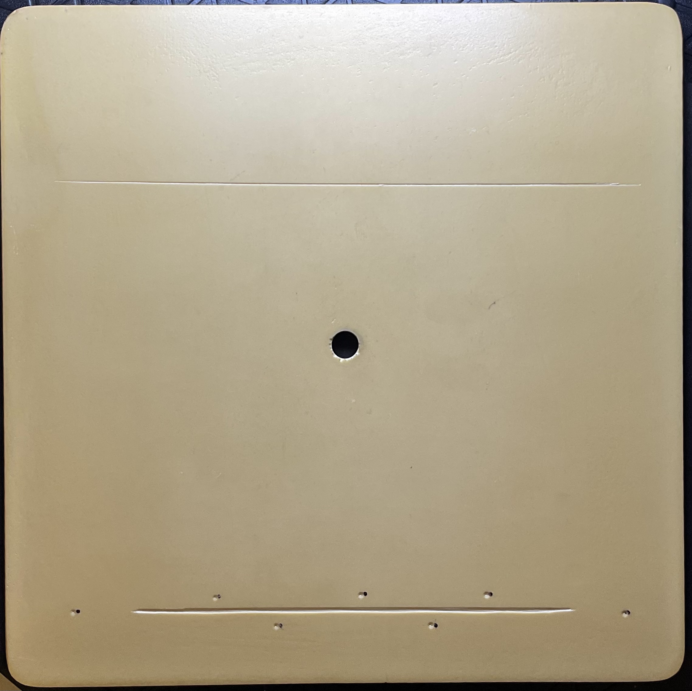
A synthetic bone plate with the following dimensions is used as a contact material:

250 mm length

250 mm width

6 mm thickness

75Shore hardness D

Synthetic bone (BP) is used as contact material for the following tool samples:

1. Standard cut flake tool sample FLT8-1 (from Lisa Schunk et al. 2021)
2. Knapped blade tool sample FLT13-1

After the first cycle of experimentation, circular marks along the cut groove are added with a center punch to aid in 3D contour matching (step #7.2 and #9.5).

Coordinate system

A coordinate system is created with ceramic beads for each tool sample. This provides reference points to relocate positions on the sample before, during and after experiments. The coordinate system is calibrated during documentation. The ceramic beads are placed a few millimeters away from the edge of each side of each tool sample.

For more details refer to the following article:

Documentation

Before and after each experiment, the tool samples and contact material are documented. Note that the contact materials are not documented before the experiment because their surface is featureless.

• Acetone is applied to the edge of the tool samples with a cotton swab for intermediate cleaning as needed throughout the documentation.

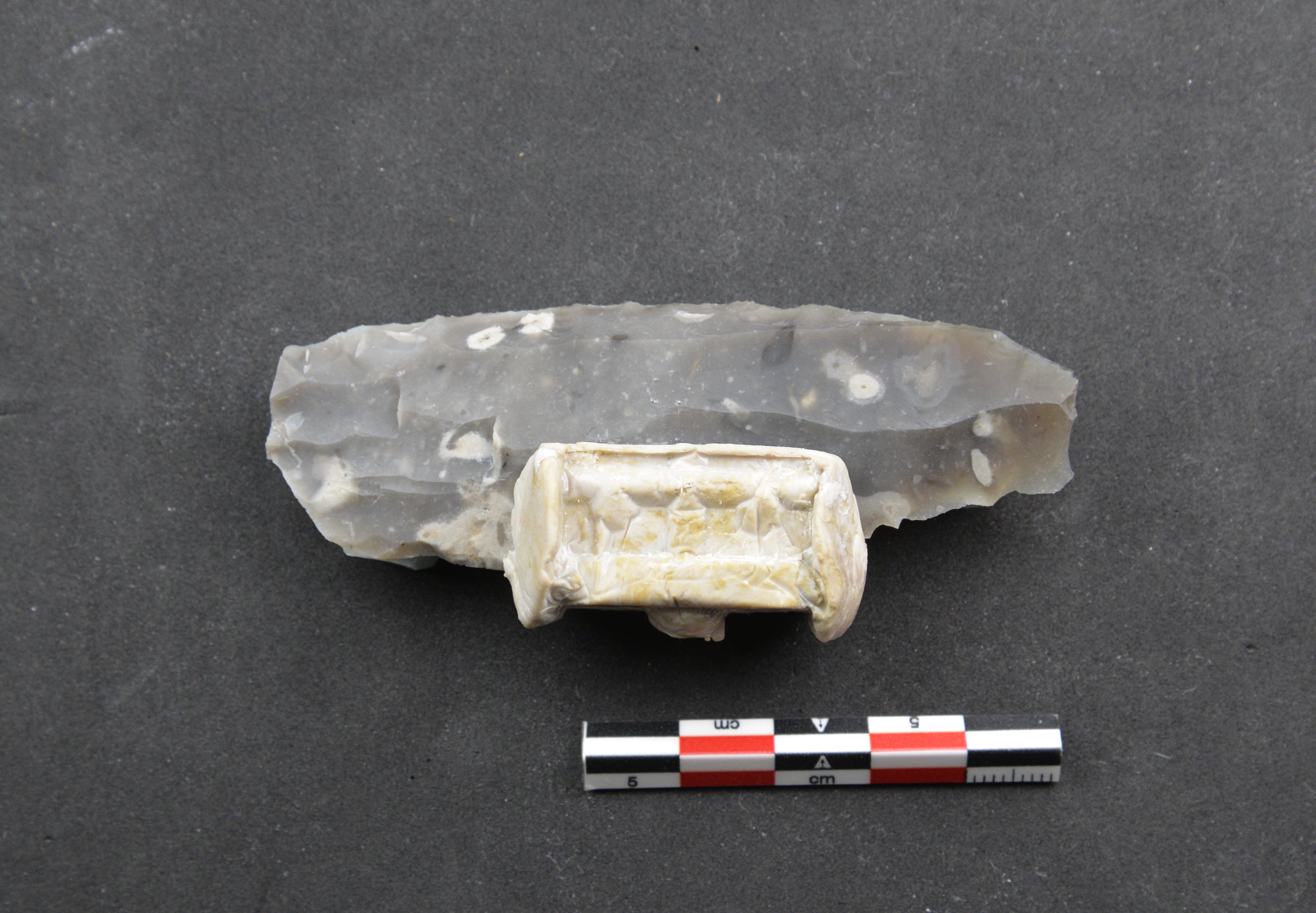
Photo

Digital photos are taken of each side (dorsal, ventral) of the tool samples to acquire general documentation images.

Equipment

Value	Label
D610	NAME
Digital camera	TYPE
Nikon	BRAND
-	SKU
https://www.nikon.com/	LINK
Objective:
AF-S NIKKOR 24-85 mm 1:3,5-4,5G ED VR

Automatic focus setting | SPECIFICATIONS |

Surface morphology documentation

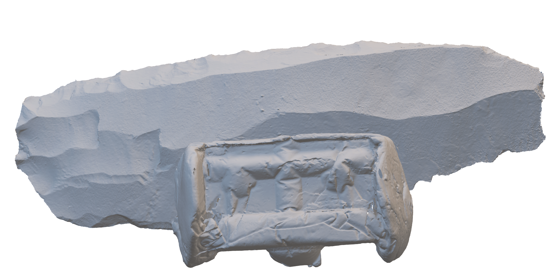
High-resolution 3D scans are created of both object (tool sample and contact material) of each sample set for archiving measurements. The scanner is turned on one hour before to avoid thermic drift. A small field of view (S-150) with a point-to-point distance of 33 µm and a measuring volume of 110 x 80 x 70 mm using following settings is used :

• The tool samples are scanned with the automatic measuring function and the turntable which takes scans while rotating 360^o. When needed, additional single scans are acquired.
• The contour matching function is used for scanning the contact materials at 90^o to the contact materials.
• The scans are merged at the working computer using the OptoCat (2020R2) software and exported as STL files.

Equipment

Value	Label
smartScan-HE R8	NAME
3D structured light scanner	TYPE
AICON	BRAND
-	SKU
S-150 FOV, resolution of 33 µm	SPECIFICATIONS

Software

Value	Label
OptoCat	NAME
Hexagon Manufacturing Intelligence Software	DEVELOPER
2020R2	VERSION

Overview images

Overview images are acquired for each side (dorsal, ventral) of the tool samples using a digital microscope Smartzoom5. The following steps are followed:

• The sample is calibrated with the coordinate beads using the 1.6x/0.1 objective.
• A 3D image of the edge is acquired with the 1.6x objective using the tile-stitching and z-stack functions.
• Settings: the ringlight brightness is identical for all images and the exposure is adjusted as needed. The blending function is activated to acquire smoother borders between the tiles.
• An EDF image of the edge is acquired and exported as CZI and PNG files.

Equipment

Value	Label
Smartzoom5	NAME
Digital microscope	TYPE
Zeiss	BRAND
https://www.zeiss.de/mikroskopie/produkte/imaging-	SKU
http://www.zeiss.com	LINK
1.6x objective; EDF-stitching images	SPECIFICATIONS

Microwear documentation

Abrasion in the form of polish (i.e., brighter and/or smoother surfaces) on the tool samples is documented with the upright light microscope (Axio Imager.Z2 Vario). The coordinate system is calibrated so that images can be layered on overview images from the digital microscope (step #7.3). The following workflow is followed:

• The coordinate beads are calibrated using the 10x objective when possible. In cases when the working distance is too small, the 5x objective is used.
• All polishes are imaged with low magnification objectives (5x or 10x) to later measure their overall size (step #14). Images are acquired using the tiles and z-stack function where needed.
• Each polished are is sampled with the 20x objective for acquiring detailed images of each polish (step #15). Images are acquired using the tiles and z-stack function where needed.

Equipment

Value	Label
Zeiss LSM 800 MAT	NAME
Confocal Laser Scanning Microscope	TYPE
Zeiss	BRAND
-	SKU
http://www.zeiss.com	LINK
Upright light microscope 5×/0.20, 10×/0.40, 20×/0.70; Bright field; Tiles and z-stack	SPECIFICATIONS

Software

Value	Label
Zen Lite (Blue Edition)	NAME
Zeiss	DEVELOPER
https://www.zeiss.com/microscopy/us/products/microscope-software/zen-lite.html	LINK
2.6	VERSION

Preservation of the edge

Molds for each side of the tool samples are collected for revisiting the state of the edge prior to experimentation:

• A generous layer of silicone is applied to the edge including the coordinate beads and a microscope slide is pressed onto the surface.
• The silicone and set for 0h 4m 0s
• The slide and silicone are removed.

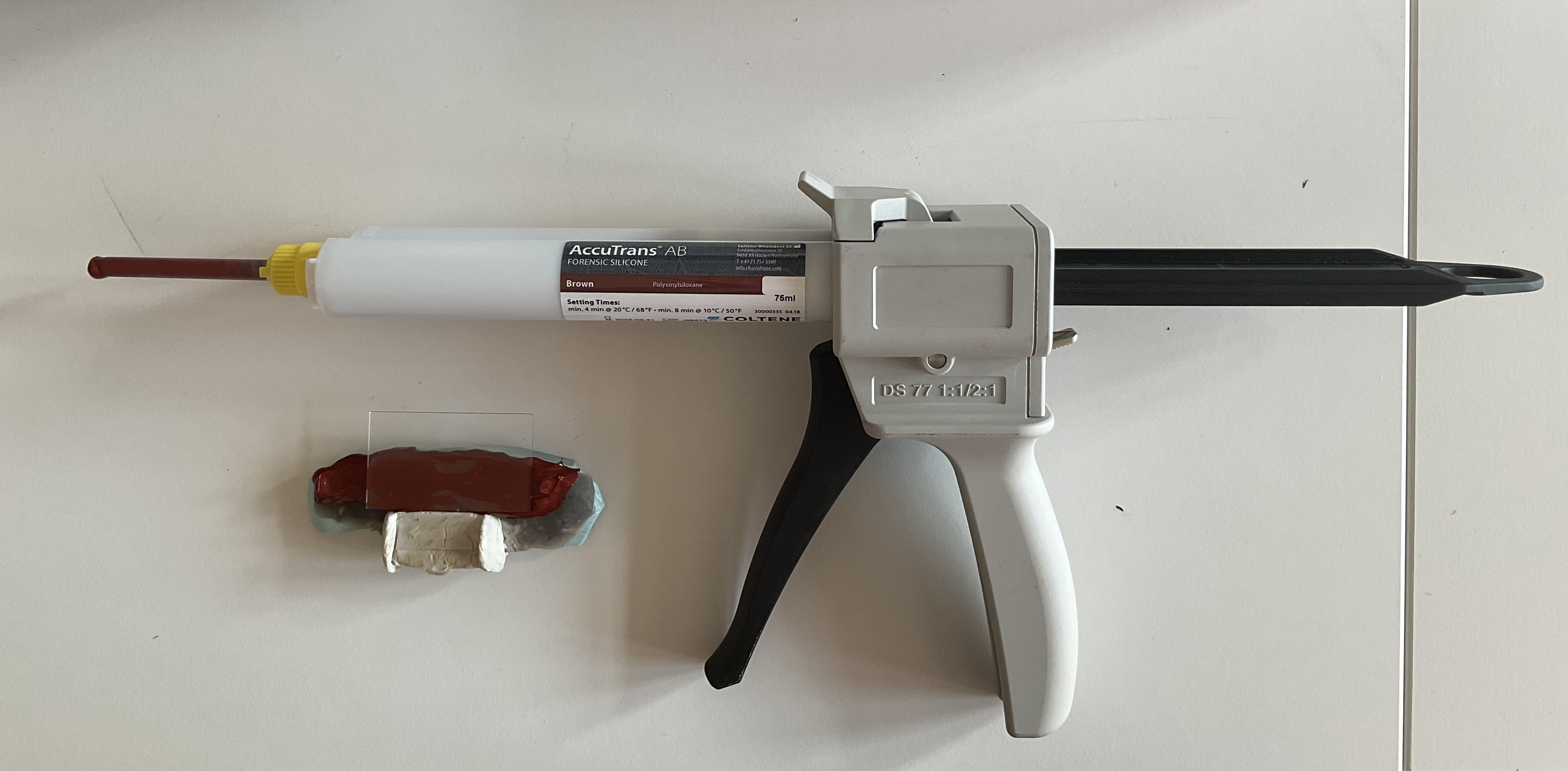
Note that for tool sample FLT8-1 (Schunk et al. 2021), a different molding material was used:

For more information on silicone molding see the following:

Citation

L. Schunk, M. Weber, I. Calandra, W. Gneisinger, J. Marreiros 2022 Comparative Study of Silicone Moulding Materials in Archaeology and the Forensic Sciences http://dx.doi.org/10.13140/RG.2.2.26648.67845

Cleaning

Right before experimentation, tool samples are cleaned to remove any residues that may have accumulated during documentation, such as from moulding.

The edge is cleaned with acetone applied with cotton swab. Fibers are removed with an air compressor.

Equipment

Value	Label
480W Silent Flüsterkompressor Druckluftkompressor	NAME
Modell: 1-480-9	TYPE
IMPLOTEX	BRAND
Artikelnummer NEW-325	SKU
https://www.implotex.de/	LINK

General settings

2000strokes of linear unidirectional cutting movements are performed for a total of four sets of experimental material. Note that one sample ran for more than 2000 strokes (FLT13-1) , due to software issues.

1. FLT 13-1 knapped blade tool sample; OFA-BP1 synthetic bone plate
2. FLT-12 knapped blade tool sample; OFA-WP1 pine wood plate
3. FLT8-1 standard cut flake tool sample; BP-I synthetic bone plate (Schunk et al. 2021)
4. FLT8-13 standard cut flake tool sample; OFA-WP1 pine wood plate

Experimental setup

A template with the following parameters for unilinear movements was programmed in the modular material tester:

5kg

140mm and 170mm for sample FLT8-1

600mm/s

4000mm/s2

10Hz

Equipment

Value	Label
Modular material tester	NAME
Inotec AP	BRAND
-	SKU
Recorded values with the time stamps: for each drive: position, speed; penetration depth with extra sensor; applied force with extra sensor; friction with extra sensor	SPECIFICATIONS

Setup sample set

The synthetic bone plate is clamped in a custom-made sample holder and fixed with a screw in the middle of the bone plate. Wood contact material is fixed with four screws on each corner.

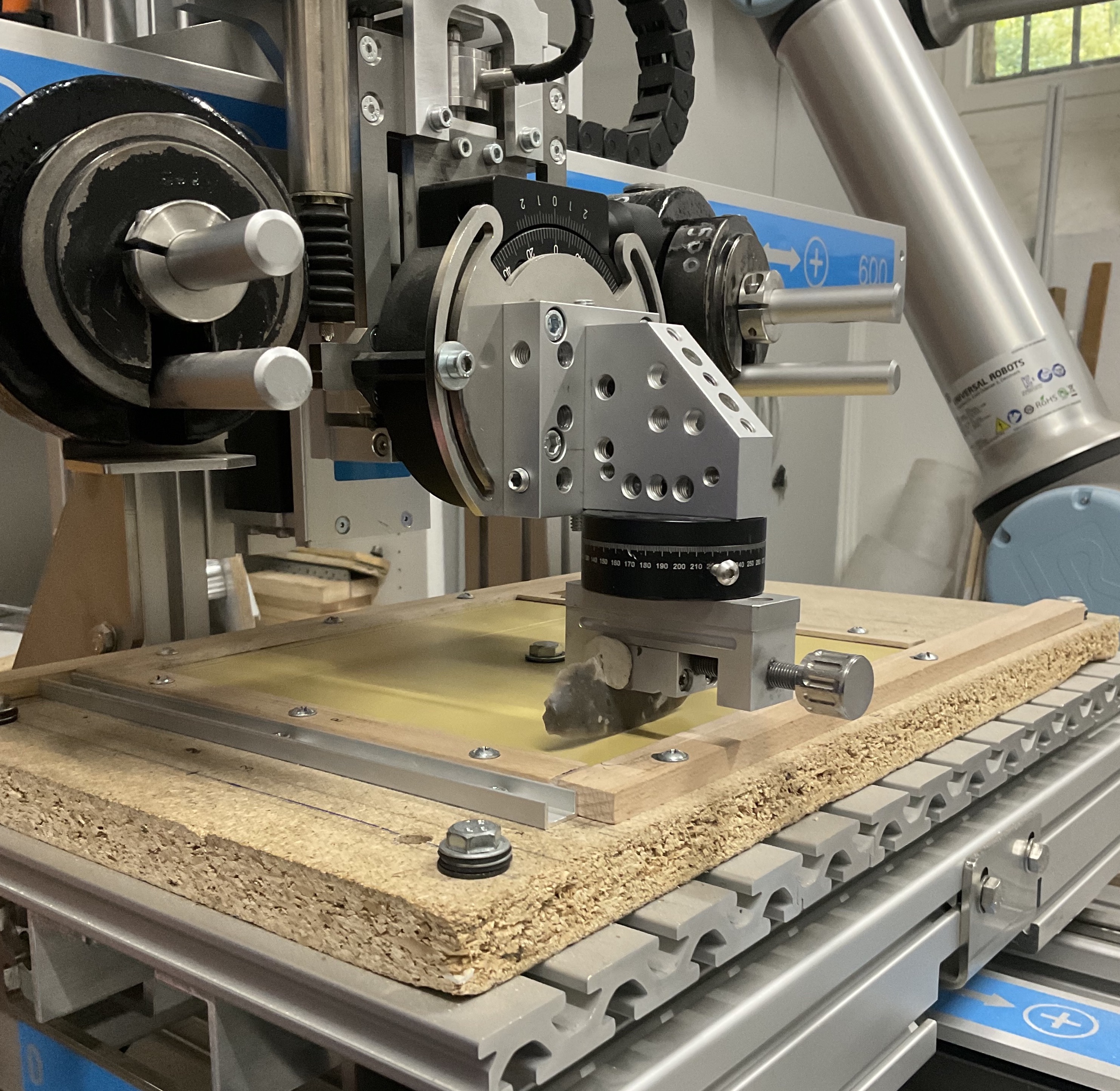
The knapped tool samples are fixed in the sample holder (SMARTTESTER®) with their sample clamps. Then, the sample holder (SMARTTESTER®) is orientated by rotating the y-axis to create the most amount of contact between the tool sample and the contact material, which depends on the curvature of the edge of the tool sample.

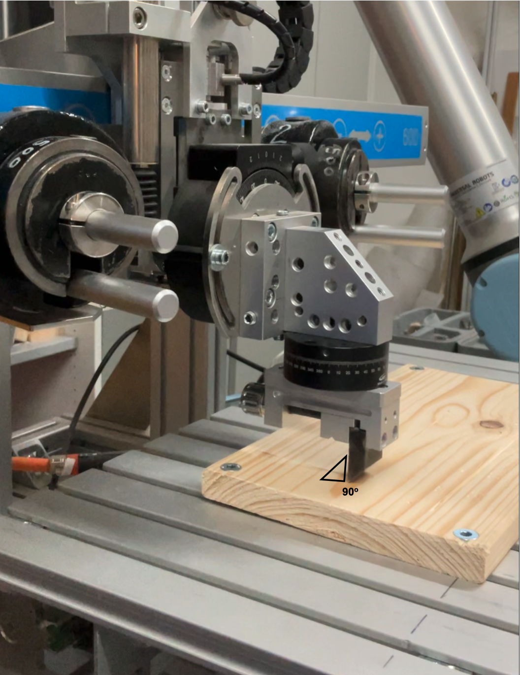
The standardised saw-cut tool samples are clamped in the sample holder (SMARTTESTER®) and manually oriented to create a 90° between the active edge of the tool sample and the contact material.

Program cutting motion

The program is identical for each experiment and was adopted from Schunk et al. 2021:

The program settings are listed here:

a) Vertical movement in the z-axis to start.

The z-value of the starting point is defined as follows: The z-drive is moved down slowly until the edge of the tool sample is in contact with the bone plate. 5 mm are added to the position of the z-drive to allow the sample to penetrate the contact material.

b) Linear movement in the x-axis for a total of 140mm . Tool sample FLT8-1 travelled 170mm .

c) Upwards vertical movement in the z-axis approx. 20mm . At this point, no contact is between the tool sample and the contact material.

d) Linear movement in the x-axis to the starting point.

e) Repeat loop for a total of 2000strokes

Note that for each experiment, five CSV files are exported corresponding to each recorded channel:

• Applied force in [N] as measured by the force sensor in the sample holder.
• Friction in [N] measured by the force sensor on the stage and the contact material.
• Penetration depth in [mm] as measured by the distance sensor in the sample holder.
• Position in [mm] of the x-drive (travel range).
• Velocity in [mm/s] of the x-drive.

FLT13-1_cutting_template.Smart

Run experiment

After both the tool sample and the contact material are fixed in the SMARTTESTER®, the program is run for a total of 2000 cutting strokes.

To avoid lubrication between residues from the contact material and the tool samples, these are removed manually with an air compressor every 50 strokes.

Equipment

Value	Label
480W Silent Flüsterkompressor Druckluftkompressor	NAME
Modell: 1-480-9	TYPE
IMPLOTEX	BRAND
Artikelnummer NEW-325	SKU
https://www.implotex.de/	LINK

3D scan of experimental setup

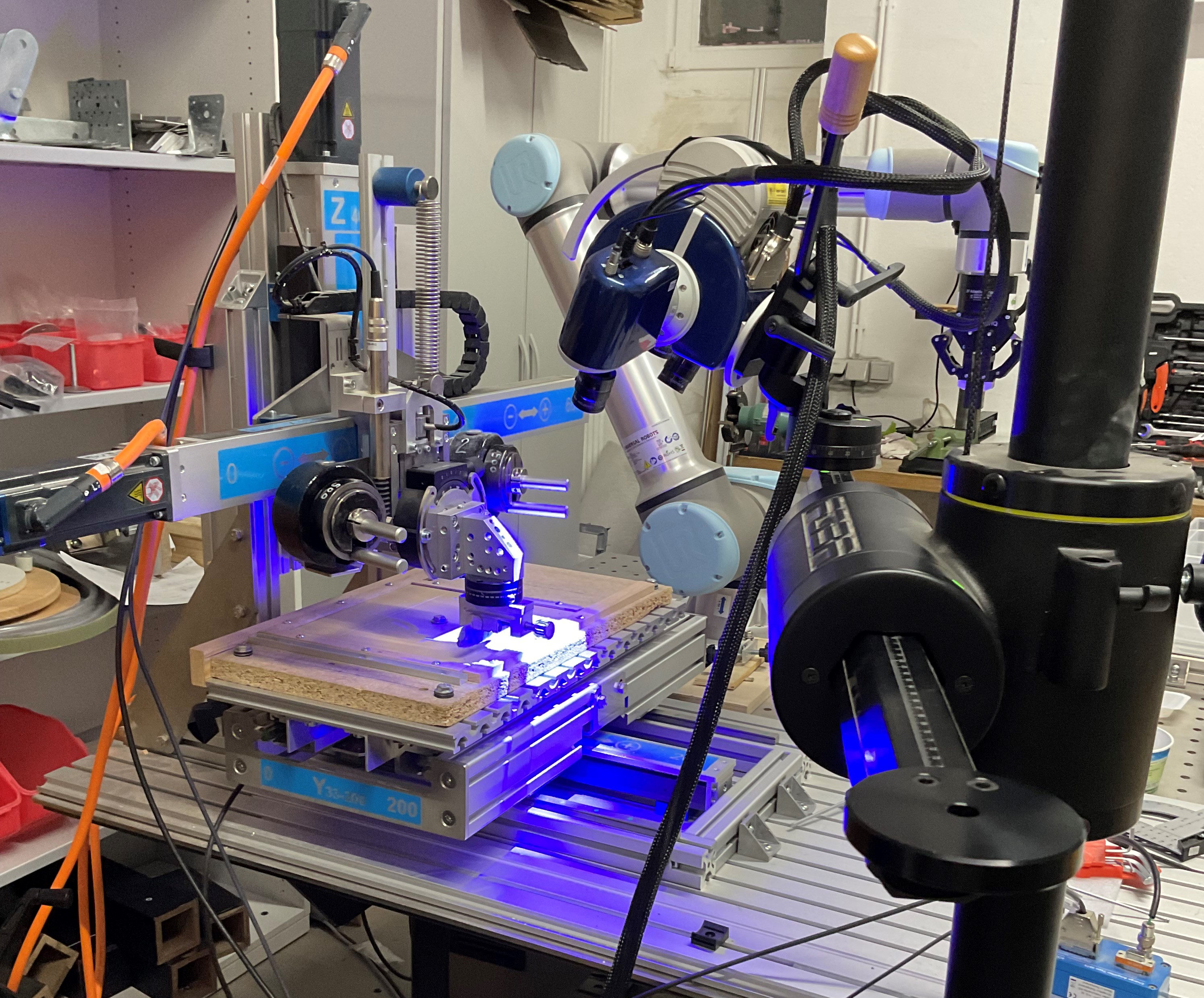
The relative position of each tool sample and contact material is scanned in situ (i.e., in the position of the starting point of the linear trajectory) directly after experimentation. This step is necessary for acquiring a proper alignment of the individual 3D scans (step #7.2) and an identical trajectory of experimentation in the OFA software (step #15). The Aicon 3D structured light scanner with a small field of view (S-150) is used for taking a series of single scans from varying angles by moving the scanning mount around the SMARTTESTER®.

Equipment

Value	Label
smartScan-HE R8	NAME
3D structured light scanner	TYPE
AICON	BRAND
-	SKU
S-150 FOV, resolution of 33 µm	SPECIFICATIONS

Cleaning

A cleaning solution is added to an ultrasonic bath, wherein each sample tool is submerged after experimentation to remove residues.

4L Tap-water

4mL

Equipment

Value	Label
Heated ultrasonic bath	NAME
Sonorex Digitec DT255H	BRAND
62083	SKU
https://ultraschall-welt.de/ultraschallreiniger/serien/bandelin-geraete/269/bandelin-sonorex-digitec-dt-255-h-5-5?c=0	LINK

40°C 0h 5m 0s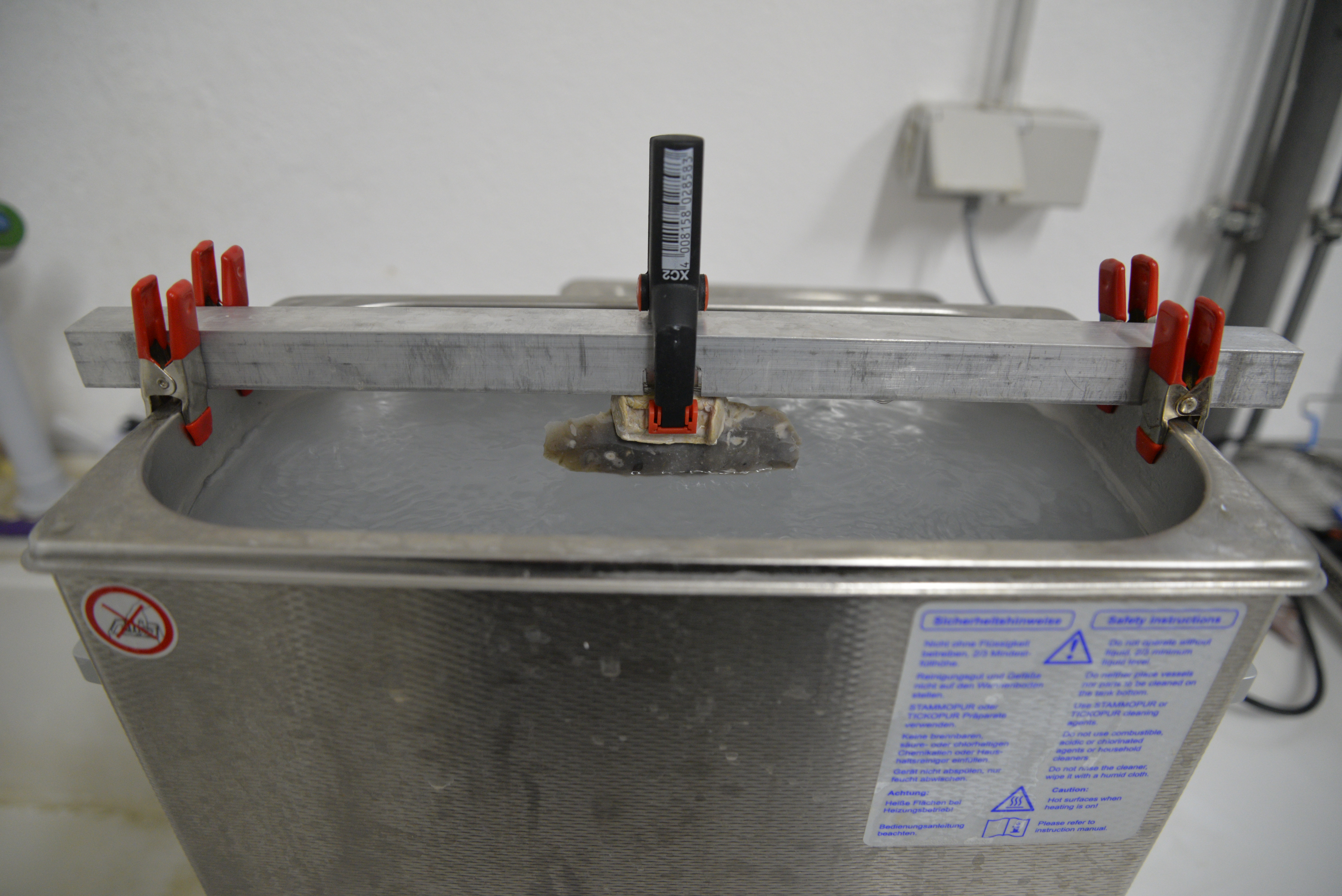

Then the edge is dried with acetone applied with cotton swabs. Cotton fibers are removed with an air compressor.

Equipment

Value	Label
480W Silent Flüsterkompressor Druckluftkompressor	NAME
Modell: 1-480-9	TYPE
IMPLOTEX	BRAND
Artikelnummer NEW-325	SKU
https://www.implotex.de/	LINK

Screening

The cleaned tool samples are screened under a stereo-microscope to check for any possible residues from experimentation.

Equipment

Value	Label
Leica M420	NAME
Stereomicroscope	TYPE
Leica	BRAND
-	SKU
http://www.leica-microsystems.com/home/	LINK
1.25 x 10 magnification	SPECIFICATIONS

Clean contact material

Contact materials are cleaned by removing abraded material in the cutting groove with an air compressor.

Equipment

Value	Label
480W Silent Flüsterkompressor Druckluftkompressor	NAME
Modell: 1-480-9	TYPE
IMPLOTEX	BRAND
Artikelnummer NEW-325	SKU
https://www.implotex.de/	LINK

Post-experiment documentation

After experimentation and cleaning, all tool samples are documented.

Image processing

Overview images of the tool samples generated from the digital microscope (step #7.3) and images of micro-wear (step #7.4) are processed using the ZEN Connect add-on for ZEN Desk add-on (v3.5 HF 9) from ZEISS.

Software

Value	Label
Zen	NAME
Zeiss	DEVELOPER
https://www.zeiss.com/microscopy/en/products/software/zeiss-zen.html	LINK
3.5 (blue editio	VERSION

Raw data from the upright light microscope (Axio Imager.Z2 Vario) micro-wear documentation are processed as follows:

• All microscope image acquisitions are imported in ZEN Desk for batch processing.
• The extended depth of focus (wavelets method without Z-Stack alignment) is applied as a batch process to microscope image acquisitions containing a z-stack.
• Acquisitions that contain multiple tiles are additionally stitched (no edge detection, minimal overlap = 5%, maximum shift = 10%, optimized comparer and best global optimizer) in batch.

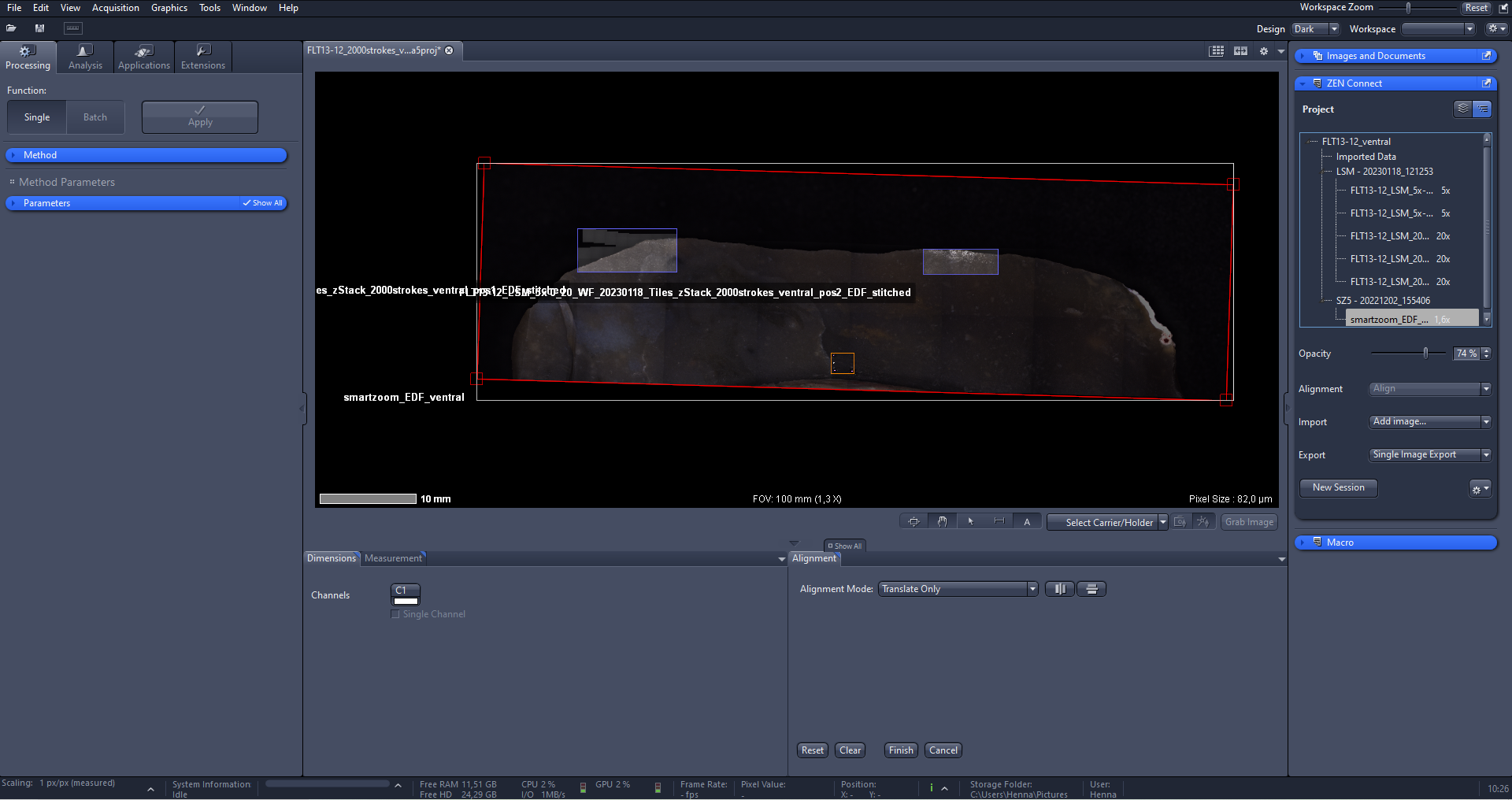
Next, all image data (i.e., overview images and use-wear documentation as described above) is processed as follows:

• All data for one side of a tool sample is imported and a project is created.
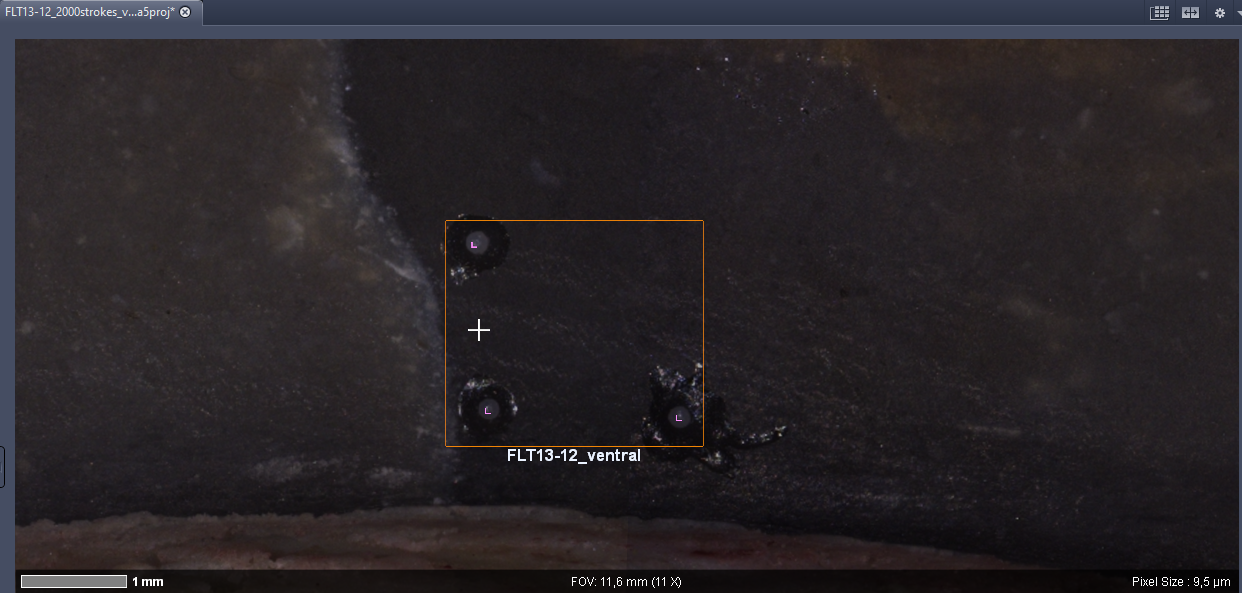
• Since coordinate beads were calibrated during acquisition in both microscopes, all images can be aligned. A sample holder is created in the project by setting a total of three markers, corresponding to the location of the coordinate beads relative to the microscope stage. The sample holders are created based on the upright light microscope images and the distance between the markers is calculated as follows: X _1–2 = X _marker2 – X _marker1 and Y _1–2 = Y _marker2 – Y _marker1* After the marker positions are set on the coordinate beads, the overview image is aligned using the translate function. The overview images needed some manual alignment because of distortion due to tilting of the knapped samples.

Measure micro use-wear

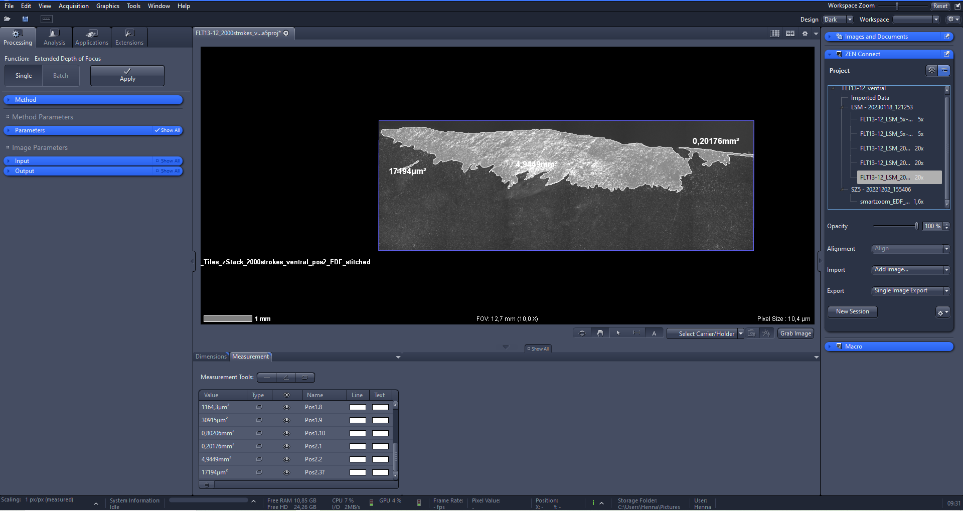
Areas of micro use-wear (polish) are marked using the polygon measurement tool to acquire an estimation of the surface area of polish. The following criteria is used for marking use-wear:

• Polish is clearly differentiable from the surrounding rock.
• Polish is bright or very bright.
• Polish is continuous.

The surface area estimations are recorded manually in a CSV table.

3D Model processing

The 3D models of each tool sample and contact materials (step #7.2) and the alignment scans (step #9.5) are processed for further use in the CloudCompare (v. 2.13.alpha, 2023) and Occlusal Fingerprint Analyser (OFA, version 2.1) software. Here, the GOM Inspect (v.2.0.1) software is used.

Software

Value	Label
GOM Software	NAME
v2.0.1	OS_VERSION
Zeiss Quality Suite	DEVELOPER
https://www.gom.com/de-de/produkte/zeiss-quality-suite?keyword=gom%20software&device=c&network=g&gclid=CjwKCAiApvebBhAvEiwAe7mHSCy3p7Njrfi46Eecqw00UuwdRp-FyW3YKv0HoFxCisPVz9kxKRpoVBoCbQEQAvD_BwE	LINK
2022	VERSION

Process 3D models for CloudCompare

1) Align 3D models

For macro use-wear (i.e., edge damage) documentation in CloudCompare, the 3D model of each tool sample before experimentation (0 strokes) and after experimentation (2000strokes) acquired in step #7.2 are processed. The workflow is as follows:

• One 3D model of a tool sample (e.g., FLT13-1 at 0strokes) is imported in GOM Inspect software as a mesh. The coordinate system is set using the set matrix function. The edge of the tool is orientated along the x-axis. The file is exported as a STL file.
• Next, the 3D model is re-imported into the software as a CAD (i.e., LFT 13-1 at 0strokes) and the second 3D model as a mesh (i.e., FLT13-1 at 2000strokes). The mesh file is aligned to the CAD using the pre-alignment and local best-fit functions. The aligned mesh is exported as an STL file.

2) Clean 3D models

The 3D models from step #13.1 are cleaned by removing additional data, filling holes and deleting mistakes. The following workflow is followed:

• The 3D models are uploaded as a mesh and cropped to remove excess and unnecessary data using the delete-by-plane function. The meshes are cropped so that only the edge of the tool sample in question is left.
• Any visible mistakes (e.g., a triangle sticking out on a flat surface) in the mesh are removed using the delete selected 3D function.
• Holes in the mesh are filled using the close holes automatically and close holes manually function. Regarding the close holes automatically function, a maximum hole size of 10 mm is selected and 1000 is selected for the maximum number of edges.
• Mistakes in the mesh are corrected using the eliminate mesh errors function.
• The cleaned meshes are exported as STLs.

Process 3D models for OFA

1) Align 3D models

The 3D models of each sample (step #7.2) are aligned to the 3D model of the relative position (step #9.5). This is necessary for creating a trajectory in the OFA software that is identical to experimentation. The workflow is as follows:

• First, the 3D model of the relative position scan is imported as a mesh. The mesh is set using the set matrix function. The cutting groove is orientated along the x-axis, the y-axis is orientated along the edge of the contact material and the z-axis is orientated along the face of the tool sample. Then, the origin is translated to be placed at the start of the cutting groove. This alignment is necessary for setting accurate scene path points in OFA (step #15). The mesh is exported as an STL.
• Next, the 3D model of the tool sample and contact material (step #7.2) are aligned one at a time to the above-orientated mesh. The orientated mesh is uploaded as a CAD and the sample 3D models (tool sample and contact material; one at a time) are imported as a mesh in the software. The tool sample mesh is aligned with the pre-alignment and local-best-fit functions, whereas the contact material mesh is aligned with the 3-point-alignment function. The 3 points are placed on prominent features of the contact material surface such as the center-punch marks. The deviations are noted before the meshes are exported as STL files.

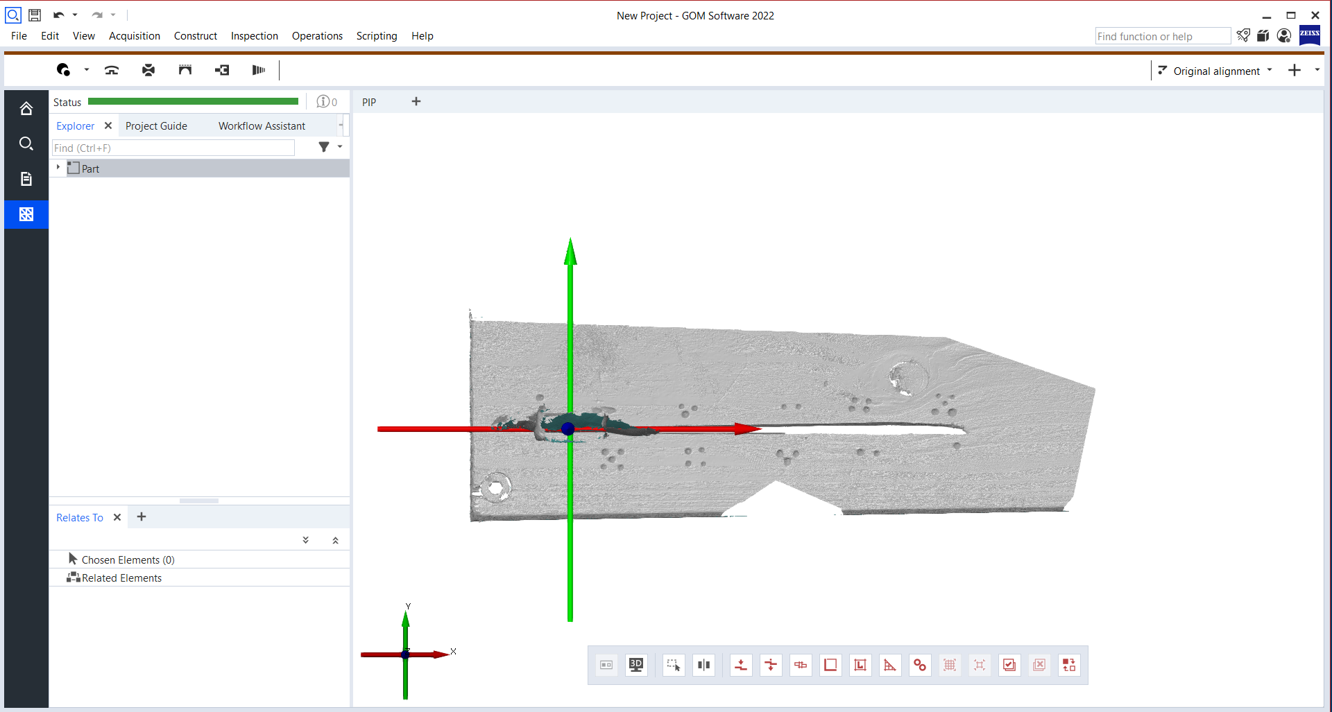
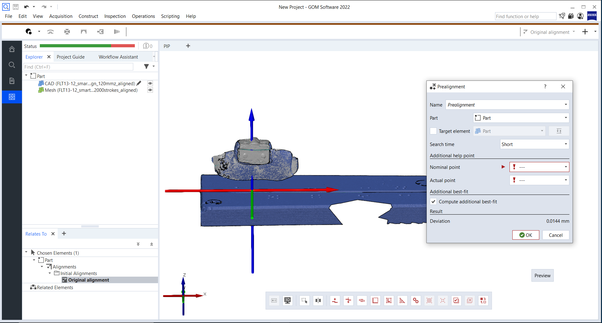
Note that for FLT8-1 and BP-1, a 90° is created between the ventral side of the tool sample and the contact material for alignment. This angle corresponds to the experimental setup from Schunk et al. 2021 where no alignment scans were taken.

2) Clean 3D models

The aligned 3D models of the tool sample and contact material are cleaned by removing additional data, filling holes and deleting mistakes in the mesh. The following workflow is identical to step 12.2. Note that for the contact material, the mesh is cropped so that only the cut groove is left.

3) Create contact between 3D models

Finally, contact between each set of cleaned 3D models is created as follows:

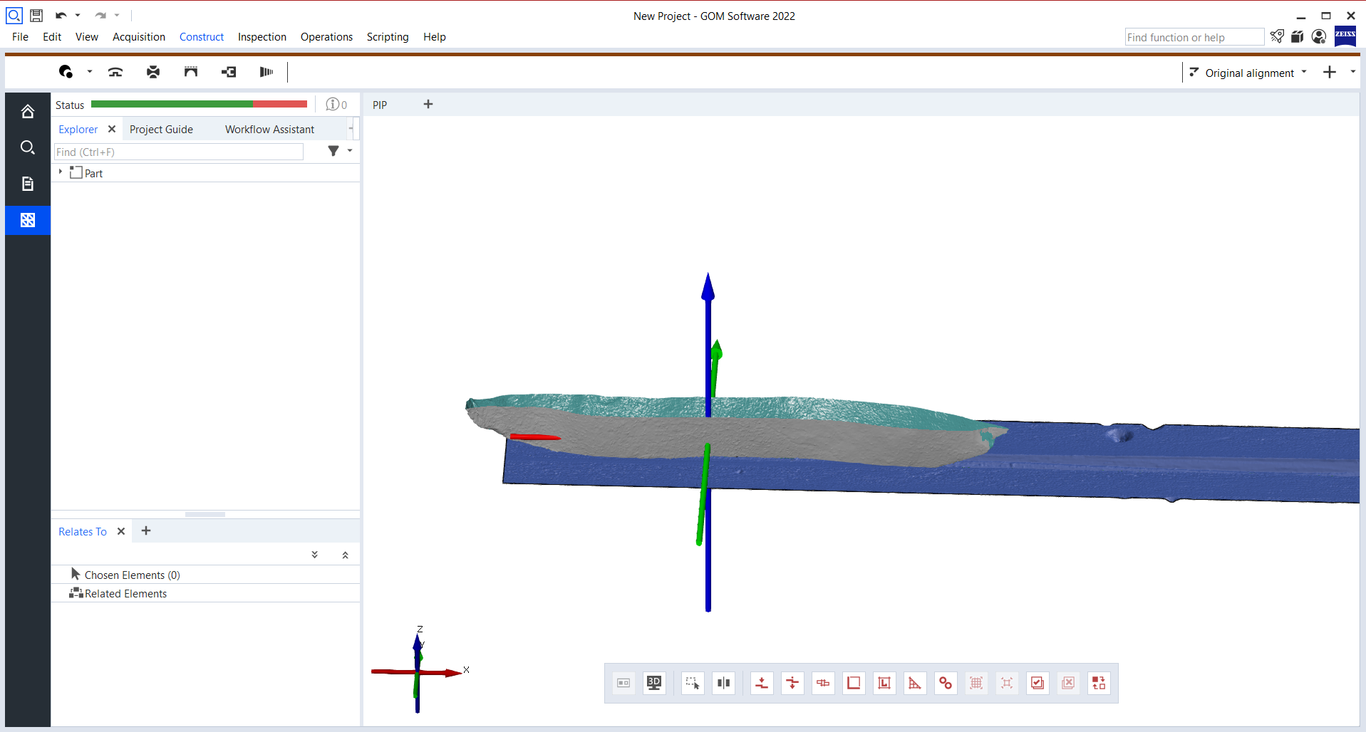
• First, the 3D model of the contact material from step #13.4 is uploaded as a CAD in the software. The 3D model of the tool sample is uploaded as a mesh.
• The mesh of the tool sample is lowered on the z-axis to create contact with the contact material CAD. The mesh is set using the set matrix function. The final z-axis position of the tool sample mesh corresponds to the z-axis position of the experimental setup. The tool sample mesh is exported in the STL file format.

CloudCompare

The C2M tool in CloudCompare is used for comparing surface deviations from mesh to mesh between each tool sample model before (0strokes) and after (2000strokes) experimentation. The data produced from this gives a comparison of the meshes before and after experimentation and therefore a visualization of edge reduction. A similar workflow to that of Nora (2021, 149) is followed and described below.

Software

Value	Label
CloudCompare	NAME
v2.13.alpha [macOS 64-bit] Compiled with Qt 5.15.2 License: GNU GPL	DEVELOPER
https://www.danielgm.net/cc/	LINK
2.13.alpha	VERSION

• First, the pre- and post experimentation STL files (step #13) of each tool sample are uploaded to CloudCompare. The models are aligned by selecting both meshes and using the match bounding-box centres and fine registration (ICP) functions under the registration tab.
• Next, the meshes are compared by selecting both and using the cloud/mesh distance function under the distance tab.
• The properties of the “registered” mesh are changed by making the colour scale visible.
• Comparison data is fetched by selecting the “registered” mesh and exporting the histogram.
• The colour scale toggle is activated and the full-screen 3D view is entered to acquire screen-shot images of the compared meshes.

Occlusal Fingerprint Analysis

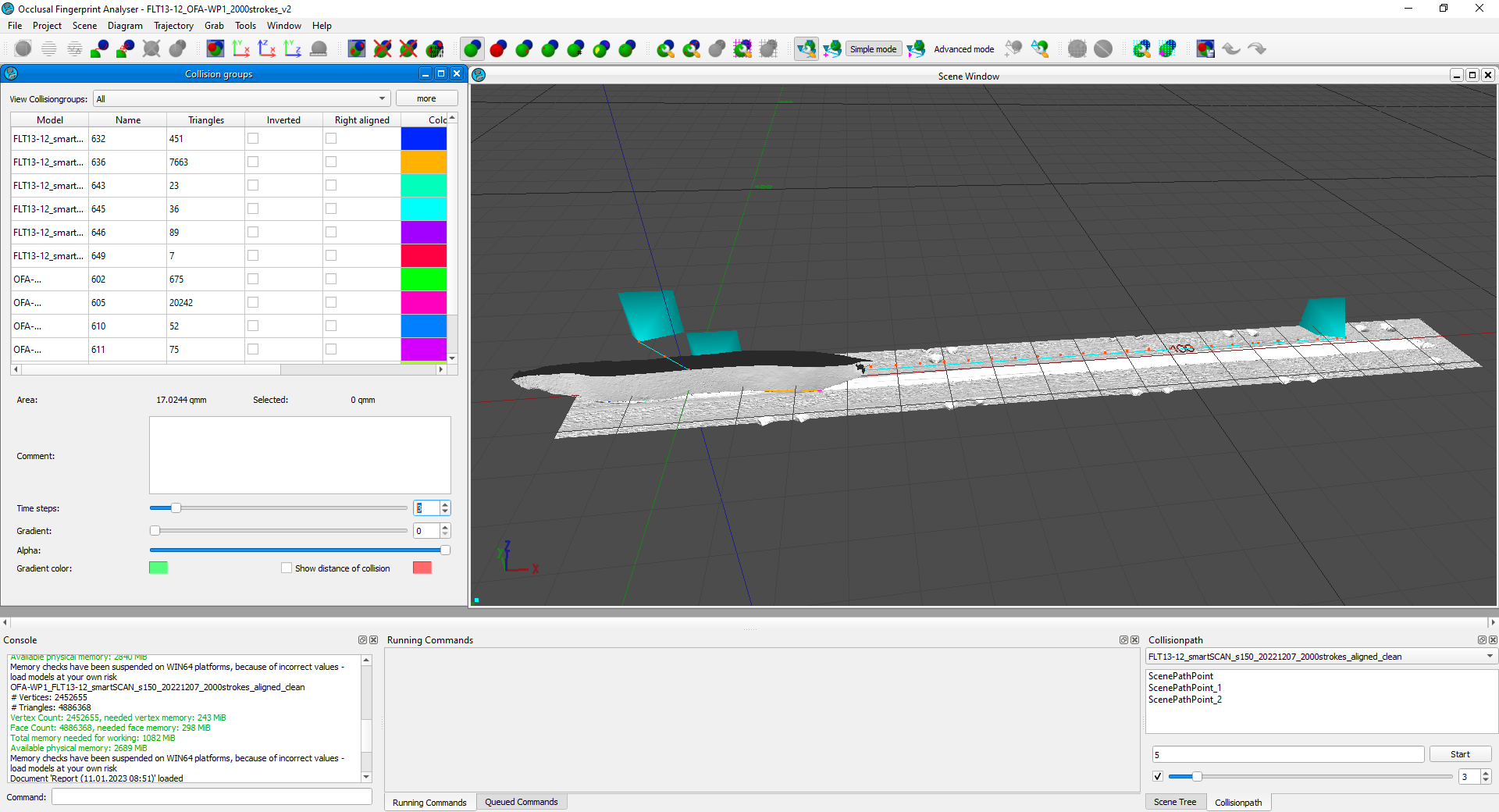
The experimental trajectory is simulated in the Occlusal Fingerprint Analyser (v.2.1) software to calculate contact areas as a comparison to the observed use-wear. The contact material (OFA-BP1, OFA-WP1) is static while each corresponding tool sample is moved in the cutting groove. The trajectory corresponds to the last (2000^th) cutting stroke from experimentation. The workflow is as follows:

• Each tool sample and the corresponding contact material STL. files (step #13) are loaded in place in the OFA software. File > load model.
• A minimum of three scene path points are set which direct the tool sample along the cutting groove. Scene tree > select tool sample > add point to path. From this position, the scene path points are translated by using the translation function. Scene tree > select scene path point > right click > translate element.

1. The first point is translated positively on the z-axis and negatively on the y-axis. The negative y translation is necessary to avoid the tool getting stuck at the cutting groove's starting point.
2. The second point always corresponds to the start position of the tool sample in the groove.
3. The third point is always at +140 mm on the x-axis which corresponds to the cutting length. For FLT8-1, a cutting length of 170 mm was set.

• Depending on the topography of the tool sample and contact material surface, it may be necessary to set further points to direct the tool sample to move in the cut groove.
• The maximum degree of break free is set to 100. Project > settings > trajectory > break free > maximum degree for break free.
• The default setting for set distance of 0.2 mm is used. Project > settings > collision > set distance.
• A step distance of 0.5 is set. Collision path > step distance.
• The trajectory is run using the start button. Collision path > start.

Software

Value	Label
Occlusal Fingerprint Analysis (OFA)	NAME
DFG research group FOR 771	DEVELOPER
https://www.ifgeo.uni-bonn.de/en/ifg_homepage/departments/paleontology/labs/vertebraten/ehemalige-forschergruppen/for-771/ofa	LINK
2.1	VERSION

Imaging contact areas

The show collision distance function gives a view of how close the collision between the two models is as a gradient. This function is activated and images with the location of contact areas on the surface of each tool sample are acquired using the grab image function. The acquisitions are exported as PNG files.

Export diagrams and reports

After each collision and trajectory, data on contact areas are collected by exporting a CSV table of the collision groups and line charts via the diagram function.

Data Analysis

All CSV files with experimental data (step #9.3) are combined into one CSV file. The sensor data recorded throughout the experimental is then analysed in R.The analysis includes descriptive statistics and plotting the variables velocity, force, penetration depth, and friction data. All packages used are cited in the R script (see #17).

Software

Value	Label
R Studio Desktop	NAME
The R Studio, Inc.	DEVELOPER
https://www.rstudio.com/products/RStudio/	LINK
1.1.463	VERSION

All data produced during this pilot study can be accessed here: DOI:

https://doi.org/10.5281/zenodo.8268058