Getting Started with LINCS Datasets and Tools
Eryk Kropiwnicki, Eryk Kropiwnicki, Alexander Lachmann, Daniel J. B. Clarke, Daniel J. B. Clarke, Avi Ma'ayan, Zhuorui Xie, Zhuorui Xie, Megan L. Wojciechowicz, Megan L. Wojciechowicz, Kathleen M. Jagodnik, Kathleen M. Jagodnik, Ingrid Shu, Ingrid Shu, Allison Bailey, Allison Bailey, Minji Jeon, Minji Jeon, John Erol Evangelista, John Erol Evangelista, Maxim V. Kuleshov, Maxim V. Kuleshov, Abhijna A. Parigi, Jose M. Sanchez, Sherry L. Jenkins
Abstract
The Library of Integrated Network-based Cellular Signatures (LINCS) was an NIH Common Fund program that aimed to expand our knowledge about human cellular responses to chemical, genetic, and microenvironment perturbations. Responses to perturbations were measured by transcriptomics, proteomics, cellular imaging, and other high content assays. The second phase of the LINCS program, which lasted 7 years, involved the engagement of six data and signature generation centers (DSGCs) and one data coordination and integration center (DCIC). The DSGCs and the DCIC developed several digital resources, including tools, databases, and workflows that aim to facilitate the use of the LINCS data and integrate this data with other publicly available data. The digital resources developed by the DSGCs and the DCIC can be used to gain new biological and pharmacological insights that can lead to the development of novel therapeutics. This protocol provides step-by-step instructions for processing the LINCS data into signatures, and utilizing the digital resources developed by the LINCS consortia for hypothesis generation and knowledge discovery. © 2022 The Authors. Current Protocols published by Wiley Periodicals LLC.
Basic Protocol 1 : Navigating L1000 tools and data in CLUE.io
Basic Protocol 2 : Computing signatures from the L1000 data with the CD method
Basic Protocol 3 : Analyzing lists of differentially expressed genes and querying them against the L1000 data with BioJupies and the Bulk RNA-seq Appyter
Basic Protocol 4 : Utilizing the L1000FWD resource for drug discovery
Basic Protocol 5 : KINOMEscan and the KINOMEscan Appyter
Basic Protocol 6 : LINCS P100 and GCP Proteomics Assays
Basic Protocol 7 : The LINCS Joint Project (LJP)
Basic Protocol 8 : The LINCS Data Portals and SigCom LINCS
Basic Protocol 9 : Creating and analyzing signatures with iLINCS
INTRODUCTION
Acronyms, Abbreviations, and Definitions
| ALS | Amyotrophic lateral sclerosis |
| CD | Characteristic Direction |
| DCIC | Data Coordination and Integration Center |
| DSGC | Data and Signature Generation Center |
| DToxS | Drug Toxicity Signature Generation Center |
| GEO | Gene Expression Omnibus |
| GCP | Global chromatin profiling |
| GTEx | Genotype Tissue-Expression Project |
| HMS | Harvard Medical School |
| iLINCS | Integrated LINCS |
| iPSC | Induced pluripotent stem cell |
| LDP | LINCS Data Portal |
| Limma | Linear Model for Microarray Analysis |
| LINCS | Library of Integrated Network-based Cellular Signatures |
| MEP | Microenvironment perturbation |
| PCCSE | Proteomic Characterization Center for Signaling and Epigenetics |
| PCR | Polymerase chain reaction |
| SMA | Spinal muscular atrophy |
| SOP | Standard Operating Procedure |
| t-SNE | t-Distributed Stochastic Neighbor Embedding |
Library of Integrated Network-based Cellular Signatures (LINCS)
Transcriptomics and other omics enable the characterization of biological processes through the identification of key molecular components and networks that govern normal physiology and disease mechanisms. The initial introduction of transcriptomics-based high-throughput drug screens has enabled the generation of gene expression profile search engines leading to new discoveries in systems pharmacology.
The establishment of the original Connectivity Map (CMAP) resource represents one of the earliest efforts to create a large reference database and search engine for human gene expression profiles (Lamb et al., 2006). Initially, CMAP contained 453 gene expression signatures, profiled with Affymetrix GeneChip microarrays, for 164 small molecules applied to four human cell lines. This resource was then expanded to contain over 7000 signatures for over 1300 compounds including most of the FDA approved drugs. Importantly, CMAP was delivered as a web-based tool to enable users to query their own signatures against the database. The first iteration of the website was widely popular, attracting thousands of users and citations from publications that utilized the resource. As a result, the NIH established the Library of Integrated Network-Based Cellular Signatures (LINCS) program to further research in the area of omics-based drug screens. For LINCS, the CMAP team at the Broad Institute set the ambitious goal of significantly expanding the original CMAP resource by utilizing a low-cost scalable transcriptomics technology called the L1000 assay (Subramanian et al., 2017).
The L1000 assay uses Luminex bead technology to measure the expression of 978 genes, from which the expression of an additional set of 11,350 genes is computationally inferred. As of 2021, the CMAP team at the Broad Institute has produced over 3 million L1000 profiles that can be converted into over 1 million unique gene expression signatures. All this data is freely available to the research community and can be accessed from several sources including the CLUE portal (Subramanian et al., 2017), SigCom LINCS (Evangelista et al., 2022), the NCBI Gene Expression Omnibus (GEO; Edgar, Domrachev, & Lash, 2002), and Google Big Query. Aside from the L1000 data, the LINCS Data Signature and Generation Centers (DSGCs) have generated a variety of other transcriptomics, proteomics, and imaging data to study the effects of microenvironment perturbations, drug combinations, neurodegenerative diseases, and genetic perturbations, with a common goal of elucidating the molecular mechanisms and pathways underlying cellular responses to each of these types of perturbations. In addition to the DSGCs, the LINCS Data Coordination and Integration Center (DCIC) has developed tools for integrating, analyzing, and visualizing LINCS data, and has led outreach efforts to support the overall goals of the program.
Here, we present nine unique protocols to guide users, with different ways to access the LINCS data, compute signatures, and use a variety of bioinformatics tools to leverage LINCS data for signature analysis and visualization. Basic Protocol 1 describes CLUE.io, a platform that provides access to the L1000, P100, and GCP data, and tools for exploring these data. Basic Protocol 2 explains how users can compute gene expression signatures using the Characteristic Direction method (Clark et al., 2014). Basic Protocol 3 guides users on how to leverage Biojupies (Torre, Lachmann, & Ma'ayan, 2018) and the Bulk RNA-seq Appyter (Clarke et al., 2021) for generating lists of differentially expressed genes for exploratory data analysis that includes L1000 queries. Basic Protocol 4 presents the tool L1000FWD, a fireworks visualization of over 17,000 selected L1000 signatures. L1000FWD provides interactive exploration of drug-induced L1000 signatures (Wang, Lachmann, Keenan, & Ma'ayan, 2018). Basic Protocol 5 introduces KINOMEscan, a kinase profiling assay, and the KINOMEscan Appyter (Clarke et al., 2021). This Appyter facilitates the visualization of KINOMEscan data and performs kinase enrichment analysis. In Basic Protocol 6, we introduce the P100 and GCP LINCS proteomics assays. Basic Protocol 7 presents tools to explore the LINCS Joint Project (LJP) data, a collaborative project that coupled transcriptomics data with cell viability assays to study drug responses in cancer cell lines (Niepel et al., 2019). Basic Protocol 8 gives an in-depth explanation of the LINCS Data Portals, which are centralized hubs for viewing, downloading, and analyzing LINCS data (Koleti et al., 2018; Stathias et al., 2019), and SigCom LINCS (Evangelista et al., 2022), a LINCS data search engine that was designed based on the findable, interoperable, accessible, and reusable (FAIR) guiding principles (Wilkinson et al., 2016). Finally, Basic Protocol 9 describes how to leverage the iLINCS web application (Pilarczyk et al., 2020) for generating and analyzing signatures from LINCS transcriptomics and proteomics data.
Basic Protocol 1: NAVIGATING L1000 TOOLS AND DATA IN CLUE.io
CLUE.io is a cloud-based platform developed by the LINCS Center for Transcriptomics and the Proteomic Characterization Center for Signaling and Epigenetics (PCCSE) DSGCs to provide access to raw and processed data generated from the L1000, P100, and GCP assays.
Necessary Resources
Hardware
Desktop or a laptop computer, or a mobile device, with a fast Internet connection
Software
- An up-to-date web browser such as Google Chrome (https://www.google.com/chrome/), Mozilla Firefox (https://www.mozilla.org/en-US/firefox/), Apple Safari (https://www.apple.com/safari/), or Microsoft Edge (https://www.microsoft.com/en-us/edge)
Accessing the L1000 data from clue.io
1.Navigate to the CLUE.io website at https://clue.io/.
Creating an account on the CLUE.io website
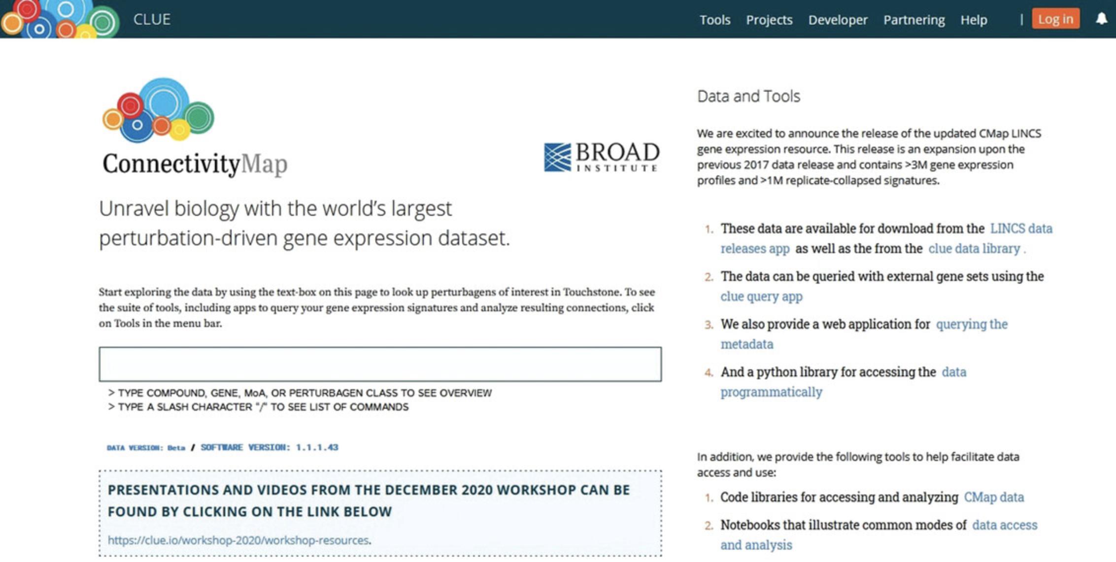
2.To access the resources on the CLUE.io site, create a free account by clicking on the Log in button at the top right of the homepage (Fig. 1), and then click the “Create an account” hyperlink. Enter your name, e-mail address, desired password, and institution, and check the box specifying that you are affiliated with a non-profit organization. Specify your research role and academic training, and then click the Create an Account button.
Logging into the CLUE.io website
3.Once you have established an account, log into the site by clicking on the Log in button at the top right of the homepage (Fig. 1), and specify your e-mail address and password. Then, click the Log in button to log into the system.
Downloading the L1000 dataset
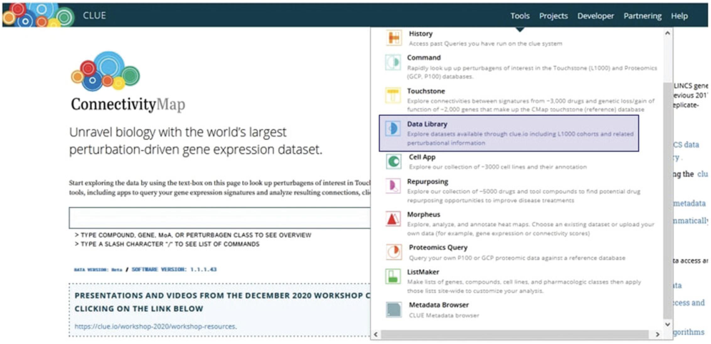
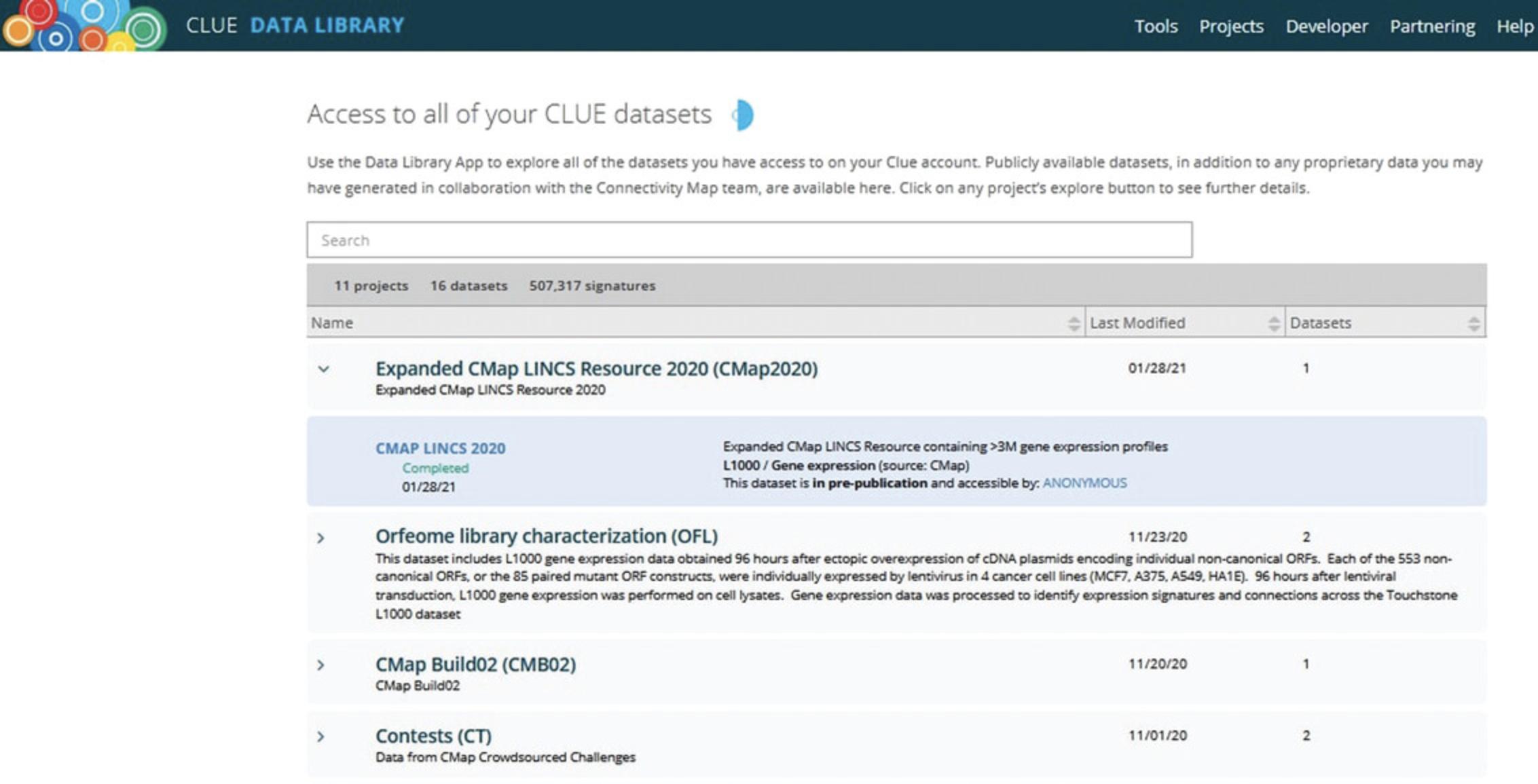
4.To access the complete L1000 data from its most recent release, select the Data Library item from the Tools menu at the top of the CLUE.io website (Fig. 2, blue shading), and then click on the “Expanded CMap LINCS Resource 2020 (CMap2020)” option in the results list (Fig. 3, blue shading) to view the components of this dataset (Fig. 4).
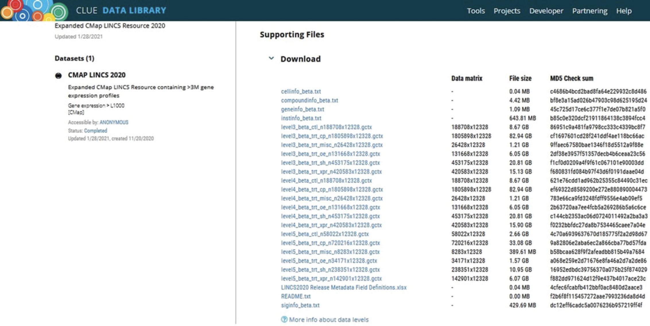
5.Files must be downloaded separately. To download each file, click on the name of the file, which serves as a download link. File sizes and dimensions are available under the “File size” and “Data matrix” columns, respectively.
Exploring the L1000 data via the CLUE.io command app
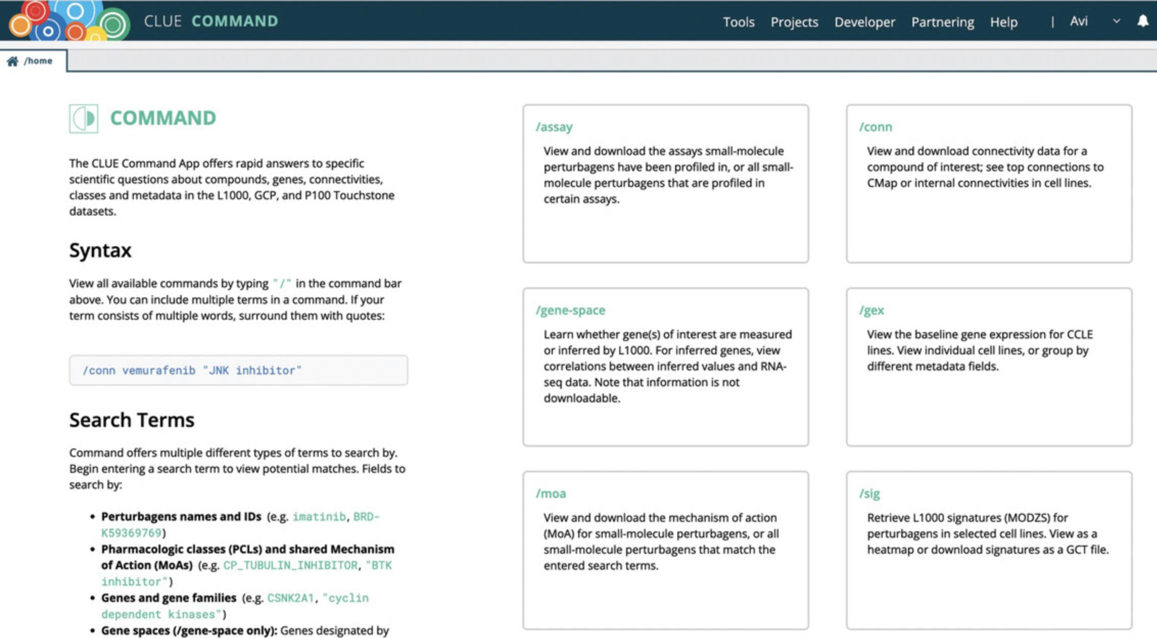
6.The CLUE Command App (Fig. 5), accessed via the Tools menu Command option, permits querying by keywords to provide detailed information about compounds, genes, classes, connectivities, and other metadata about the L1000 data and the P100 and GCP proteomics data.
-
Use the/assayoption to view and download the assays in which small-molecule perturbagens have been profiled, as well as the complete set of all small-molecule perturbagens that have been profiled with a selected assay.
-
Use the/gene-spaceoption to return information about whether genes of interest are measured or inferred by L1000.
-
Use the/moaoption to query a mechanism of action (MoA) and return all matching small molecules.
-
Using the/targetoption permits viewing and downloading target genes for queried small-molecule perturbagens, as well as all small-molecule perturbagens that match the queried terms.
-
Use the/connoption to query connectivity data for a compound and view top connections in the CMap data as well as internal connectivities in cell lines.
-
Use the/gexoption to view the baseline gene expression for Cancer Cell Line Encyclopedia (CCLE) cell lines (Barretina et al.,2012). View cell lines individually or in groups based on selected metadata fields.
-
Use the/sigoption to query L1000 signatures in Level 5 moderatedz-score format for specific perturbagens. The results are returned as a heatmap and can be downloaded as a GCT file.
Basic Protocol 2: COMPUTING SIGNATURES FROM THE L1000 DATA WITH THE CD METHOD
The L1000 Level 3 dataset can be downloaded and used to compute signatures for specific drugs and small molecules. This protocol describes the process of computing signatures from the Level 3 L1000 dataset using the Characteristic Direction (CD) method (Clark et al., 2014).
Necessary Resources
Hardware
Desktop or a laptop computer, or a mobile device, with a fast Internet connection
Software
- An up-to-date web browser such as Google Chrome (https://www.google.com/chrome/), Mozilla Firefox (https://www.mozilla.org/en-US/firefox/), Apple Safari (https://www.apple.com/safari/), or Microsoft Edge (https://www.microsoft.com/en-us/edge)
- Python 3.8+ (https://www.python.org/downloads/)
- A code editor, such as Microsoft Visual Studio Code (https://code.visualstudio.com/)
- The maayanlab-bioinformatics Python package (https://github.com/MaayanLab/maayanlab-bioinformatics)
Importing L1000 data
1.Download the following required files from the LINCS data releases app (https://clue.io/releases/data-dashboard). Save all files in the same directory as the processing script, if applicable.
- L1000 metadata for Level 5 signatures (siginfo_beta.txt)
- L1000 metadata for Level 3 signatures (instinfo_beta.txt)
- L1000 gene metadata (geneinfo_beta.txt)
- L1000 Level 3 data (level3_beta_all_n3026460 × 12328.gctx).
The GCTX file format is an HDF5-based format for storing dense matrices; it is widely used for storing the CMAP data (Enache et al., 2019). To better understand the different levels of L1000 data, please see the Critical Parameters section.
2.Define the signature of interest by cell line, perturbagen name, perturbation time, and perturbation dose. For example, the cell line A549, the drug dexamethasone, the time point 24 hr, and the concentration 10 µM would constitute a single signature.
Pre-processing data
3.Extract and store in separate tables the row names, column names, and data matrix from the Level 3 GCTX file. The row names are probe IDs that each correspond to a gene, while the column names are instance IDs corresponding to individual replicate instances of a perturbation. Each value in the 2-dimensional data matrix contains the quantile normalized expression level for a given gene in the given instance.
4.Store the batch IDs for all signatures in the signature metadata file. The batch ID is simply the text that comes before the colon in each signature ID. For example, given the signature ID “AML001_CD34_24H:BRD-A03772856:0.37037”, the corresponding batch ID would be “AML001_CD34_24H”.
5.Store the batch IDs for all perturbation instances in the instance metadata file by extracting the first three underscore-delimited terms from each sample_id. For example, given the sample ID “ERG013_VCAP_72H_X3_B11”, the batch ID would be “ERG013_VCAP_72H”.
Computing signatures with the Characteristic Direction method
6.Identify the signature of interest in the dataset by matching the cell line from step 2 to the cell_iname column, the perturbagen name to pert_iname, the timepoint to pert_itime, and the dose to pert_idose.
7.Use the distil_ids column to identify the instance IDs corresponding to the signature of interest, then slice those instances from the Level 3 GCTX file, which will be the “treatments”. Store the treatment matrix.
8.Filter the instance metadata by the batch ID corresponding to the signature of interest, then remove the treatment instances. The remaining sample IDs consist of all other instances in the batch excluding those corresponding to the treatment, and these samples will serve as “controls”. Slice these instances from the Level 3 GCTX file, and store as the control matrix.
9.Run the Characteristic Direction (CD) method on the treatment data and the control data. The method is implemented in several languages, and the code can be accessed from https://maayanlab.net/CD/; however, the simplest way is to use the maayanlab-bioinformatics Python package (https://github.com/MaayanLab/maayanlab-bioinformatics) that includes a Characteristic Direction function. The result is a vector in which each entry represents a gene and its associated CD coefficient (Clark et al., 2014).
Obtaining differentially expressed genes from the signature
10.Compute the 2-tailed z- scores and p- values for each coefficient in the CD results vector. Map the row IDs stored in step 3 to each coefficient and its p- value using the gene metadata file; the gene_id column provides the index of each gene in the vectors, and the gene_symbol column gives the common gene symbol corresponding to that index.
11.Identify all genes that correspond to a CD coefficient GREATER than 0 and a p- value < the chosen alpha. These are the up-regulated genes in the signature.
12.Identify all probe IDs that correspond to a CD coefficient LESS than 0 and a p- value < the chosen alpha. These are the down-regulated genes in the signature.
Basic Protocol 3: ANALYZING LISTS OF DIFFERENTIALLY EXPRESSED GENES AND QUERYING THEM AGAINST THE L1000 DATA WITH BioJupies and the BULK RNA-seq APPYTER
BioJupies (Torre et al., 2018) and the Bulk RNA-seq Appyter (Clarke et al., 2021) are two web-based platforms developed by the LINCS DCIC to produce customized and interactive Jupyter notebooks for RNA-seq analysis. The BioJupies platform (Torre et al., 2018) generates comprehensive Jupyter Notebook reports from user-inputted raw or processed RNA-seq data, including RNA-seq data fetched from GEO (Edgar et al., 2002) and GTEx (GTEx Consortium, 2020). Each generated notebook report can be downloaded and shared. Each automatically generated notebook is stored persistently in the cloud and is made accessible via a unique URL. BioJupies contains several analysis tools that fall under four categories: exploratory data analysis, differential expression analysis, enrichment analysis, and small molecule query. The Bulk RNA-seq Appyter is also an online web-based application that provides an interface for users to upload processed RNA-seq count data files. Then, the Appyter automatically generates Jupyter Notebook–based reports that contain analysis and visualization of the uploaded data with principal component analysis (PCA), differential gene expression analysis, and L1000 small molecule search. The Appyter reports are similar to the analyses provided with BioJupies. Both have user-friendly interfaces for uploading and submitting data, selecting computational tools, and customizing tool parameters. This basic protocol demonstrates how to use these two platforms to analyze data from published RNA-seq gene expression studies, including querying the computed signature against the L1000 data for prioritizing small molecules that can reverse or mimic the expression of the input gene expression signatures.
Necessary Resources
Hardware
Desktop or a laptop computer, or a mobile device, with a fast Internet connection
Software
- An up-to-date web browser such as Google Chrome (https://www.google.com/chrome/), Mozilla Firefox (https://www.mozilla.org/en-US/firefox/), Apple Safari (https://www.apple.com/safari/), or Microsoft Edge (https://www.microsoft.com/en-us/edge)
Submitting data to BioJupies
1a. Visit https://maayanlab.cloud/biojupies/ from your web browser (Fig. 6).
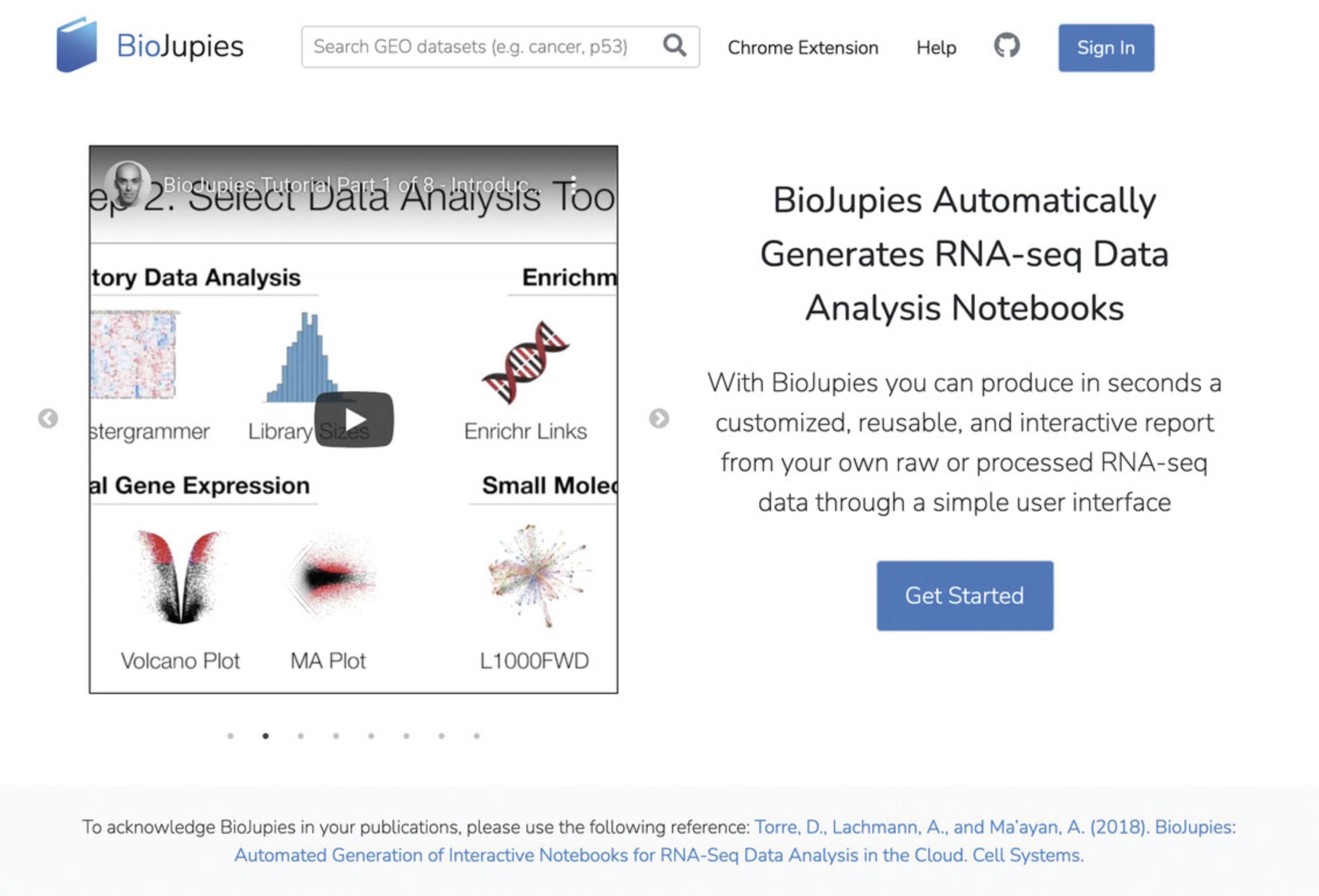
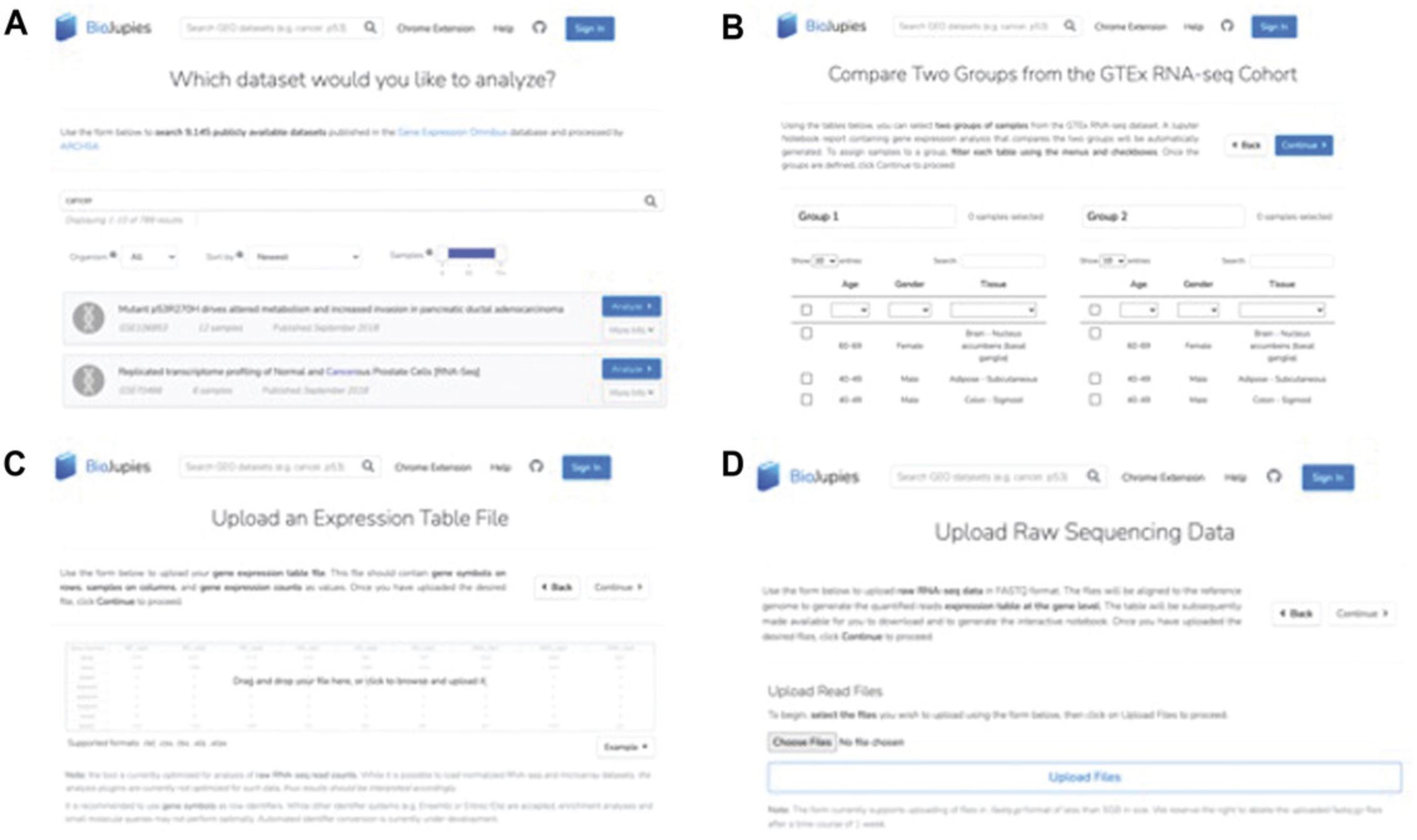
2a. Click the “Get started” button to submit data. User-inputted raw or processed data, as well as data from GEO (Edgar et al., 2002) and GTEx (GTEx Consortium, 2020), can be submitted (Fig. 7).
- To submit to BioJupies data published in GEO, select “Published Data”, then select the GEO option. Choose from 9145 processed datasets by searching by keyword, filtering by organism, or filtering by number of samples. Select one of the search results by clicking “Analyze” (Fig. 7A). As an example, we use the GEO Series GSE88741 as the input data.
- To submit data from the GTEx portal for analysis with BioJupies: select “Published Data”, then select the GTEx option. Select two groups of samples by filtering each table and checking the samples to include, then click “Continue” (Fig. 7B).
- To submit your own gene expression table (TXT, CSV, TSV, XLS, or XLSX file formats): select “Your Data”, then select “Gene Expression Table”. Either drag and drop your gene expression data file or click to browse and upload. Select “Continue” when finished. Label the sample groups manually or upload a metadata file (see example for proper formatting of your metadata file), then press “Continue” (Fig. 7C).
- To submit your own raw sequencing data: select “Your Data”, then select “Raw Sequencing Data”. Upload your data by clicking “Choose Files”, selecting your files, and clicking “Upload Files”. Note that uploaded files should be saved as fastq.gz format, must be less than 5 GB, and may be deleted after 1 week (Fig. 7D).
It is recommended to create an account when uploading FASTQ files. The alignment results will be saved in your account, so you do not have to repeat the alignment process, which can take several hours.
Querying signatures against the L1000 data with BioJupies
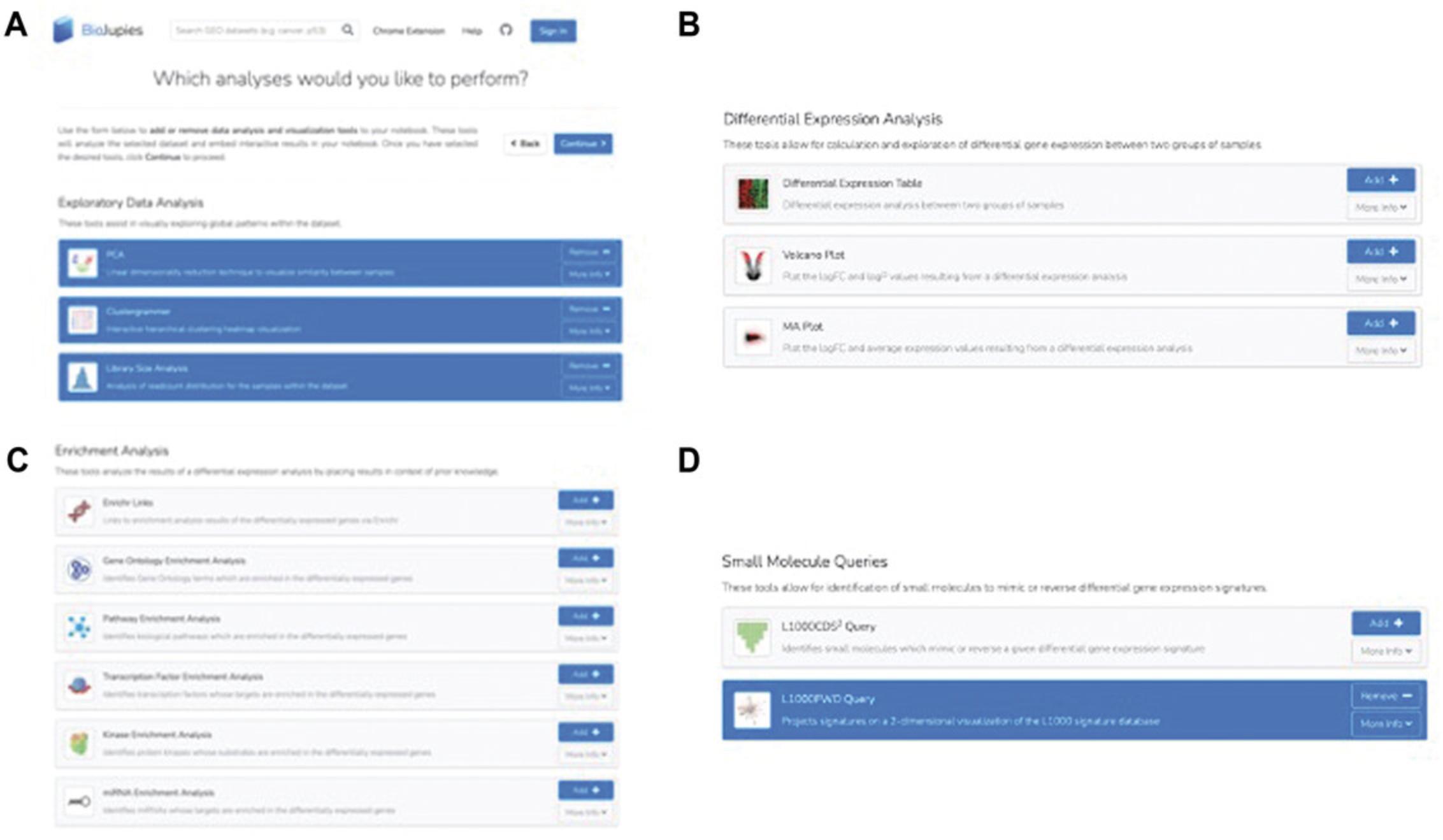
3a. The analysis page of BioJupies enables the addition or removal of data analysis tools and visualizations from the generated Jupyter Notebook report (Fig. 8). Analysis tools fall under four categories: exploratory data analysis, differential expression analysis, enrichment analysis, and small molecule queries. These tools can also be selected under their respective headers by clicking “Add”.
- Exploratory data analysis tool options include PCA , a linear dimensionality reduction technique to visualize sample similarity; Clustergrammer , an interactive hierarchical clustering heatmap visualization (Fernandez et al., 2017); and Library Size Analysis , which is analysis of the read-count distribution for samples in the dataset (Fig. 8A). In this example, we select all three options by clicking “Add”.
- Differential expression analysis tool options include Differential Expression Table (differential expression analysis between two groups of samples), Volcano Plot (plots logFC and logP values from differential expression analysis), and MA Plot (plots logFC and average expression values from differential expression analysis; Fig. 8B).
- Enrichment analysis tool options include Enrichr , which produces links to enrichment analysis results of differentially expressed genes (Kuleshov et al., 2016); Gene Ontology Enrichment Analysis , which identifies Gene Ontology terms enriched in the differentially expressed genes based on Enrichr analysis; Pathway Enrichment Analysis , which identifies biological pathways enriched in the differentially expressed genes; Transcription Factor Enrichment Analysis , which identifies transcription factors whose targets are enriched in the differentially expressed genes; Kinase Enrichment Analysis , which identifies protein kinases whose substrates are enriched in the differentially expressed genes; and miRNA Enrichment Analysis , which identifies micro-RNAs whose targets are enriched in the differentially expressed genes (Fig. 8C).
- Small molecule query options include L1000CDS2 , which identifies small molecules that mimic or reverse the provided signature (Duan et al., 2016), and L1000FWD (Wang et al., 2018), which projects the provided signature onto a 2-D fireworks visualization that projects the L1000 signature database (Fig. 8D). In this example, we select “L1000FWD Query” by clicking “Add”.
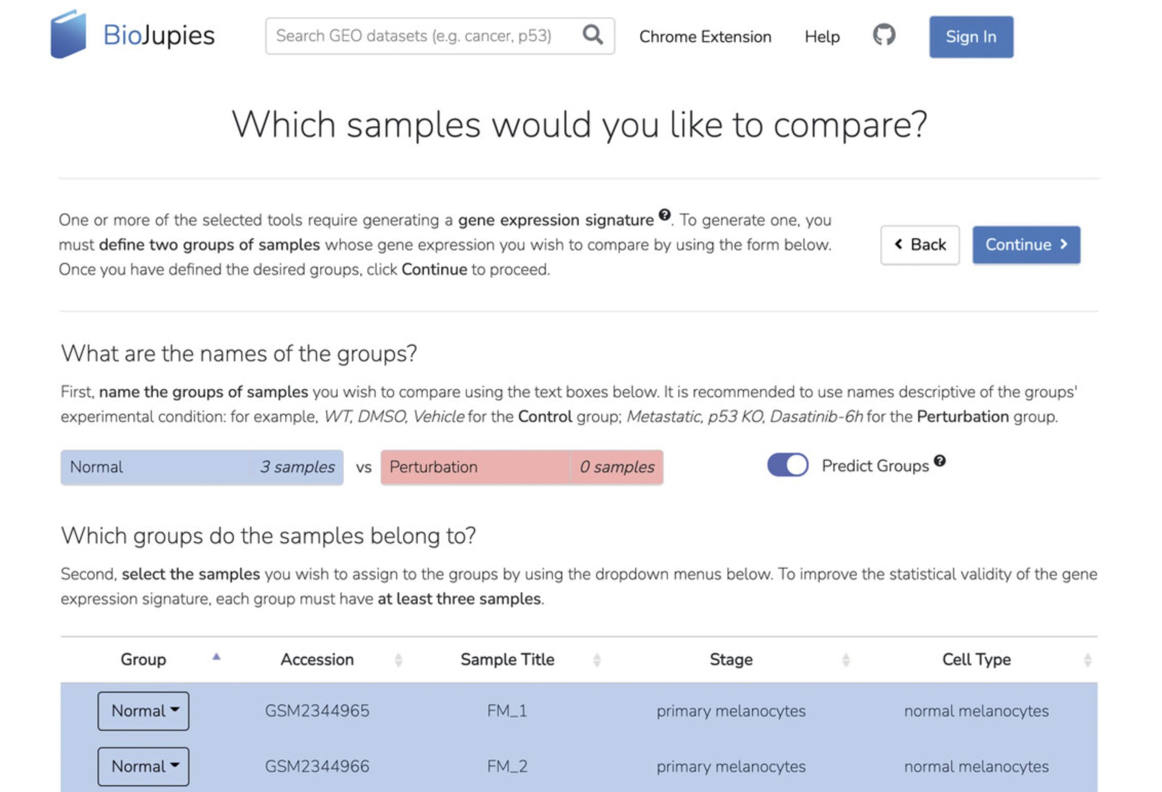
4a. On the “Which samples would you like to compare?” page, enter the names for the two groups to compare if desired, then manually label each sample with its group name. Alternatively, select “Predict Groups” to automatically classify samples based on their names. In the example, we have selected “Predict Groups”. Click “Continue” once you have selected samples into the two groups that you wish to compare (Fig. 9).
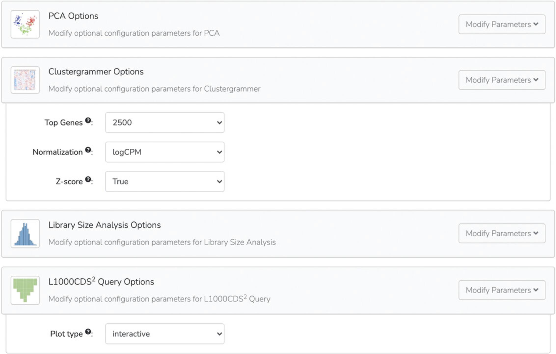
5a. On the “Review and Submit” page, customize your input parameters by selecting “Modify Parameters” and then make your desired changes. In the example, we have set the Clustergrammer settings as follows: Top Genes = 2500, Normalization = logCPM, and Z- score = True (Fig. 10). Depending on the features selected in step 3, each section will have various parameters. Click “Generate Notebook” when done.
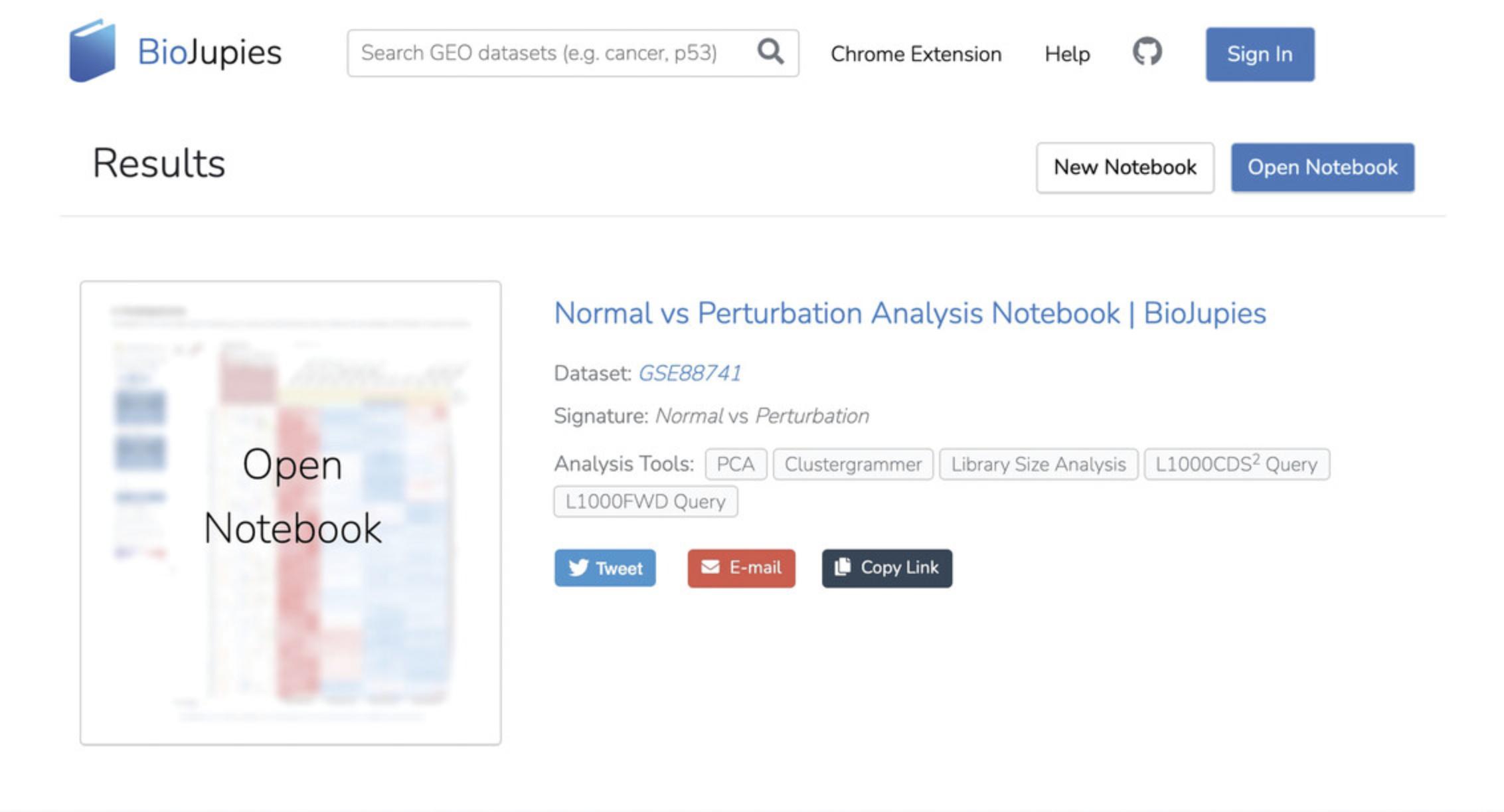
6a. Once the notebook has been generated, the “Results” page will appear. The notebook can be opened by clicking the notebook name or the “Open Notebook” buttons. The notebook can also be shared using the “Tweet”, “Email”, and “Copy Link” buttons (Fig. 11).
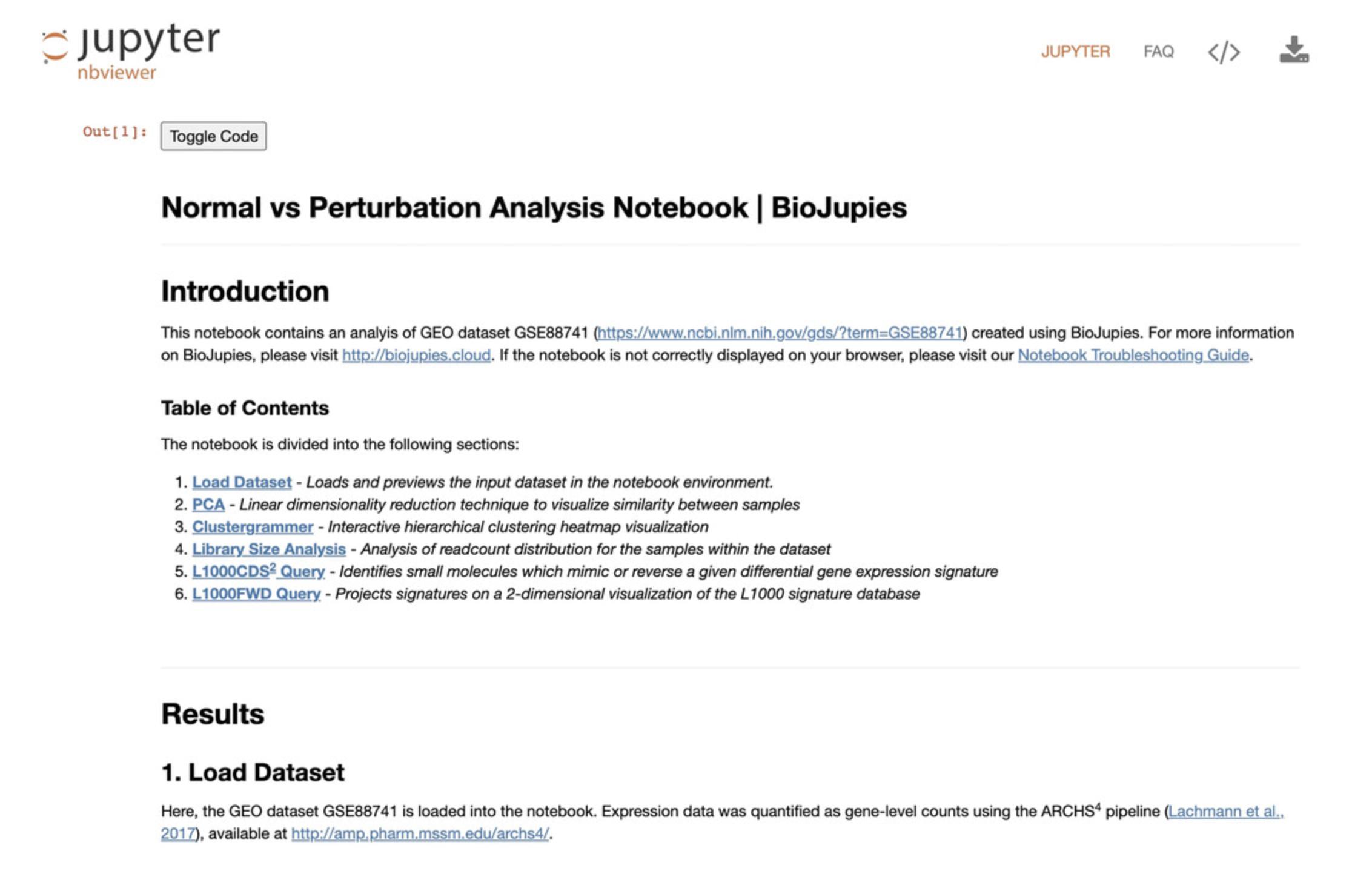
7a. With the notebook opened, a table of contents will be displayed. Select the link to any section to view each respective analysis (Fig. 12). The notebook can be downloaded by clicking the download icon in the upper right corner and clicking “Save Link As…”; this will prompt a pop-up window to save the notebook as an IPYNB file.
Submitting data to the Bulk RNA-seq Appyter
1b. Visit https://appyters.maayanlab.cloud/#/Bulk_RNA_seq in your web browser (Fig. 13).
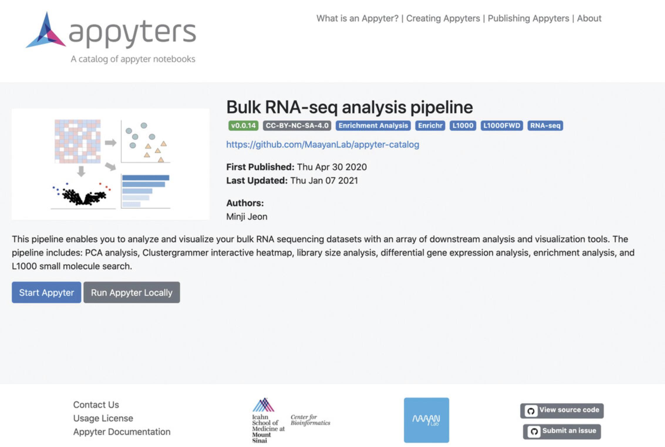
2b. Click the “Start Appyter” button. A page for selecting and customizing data and tools will be displayed.
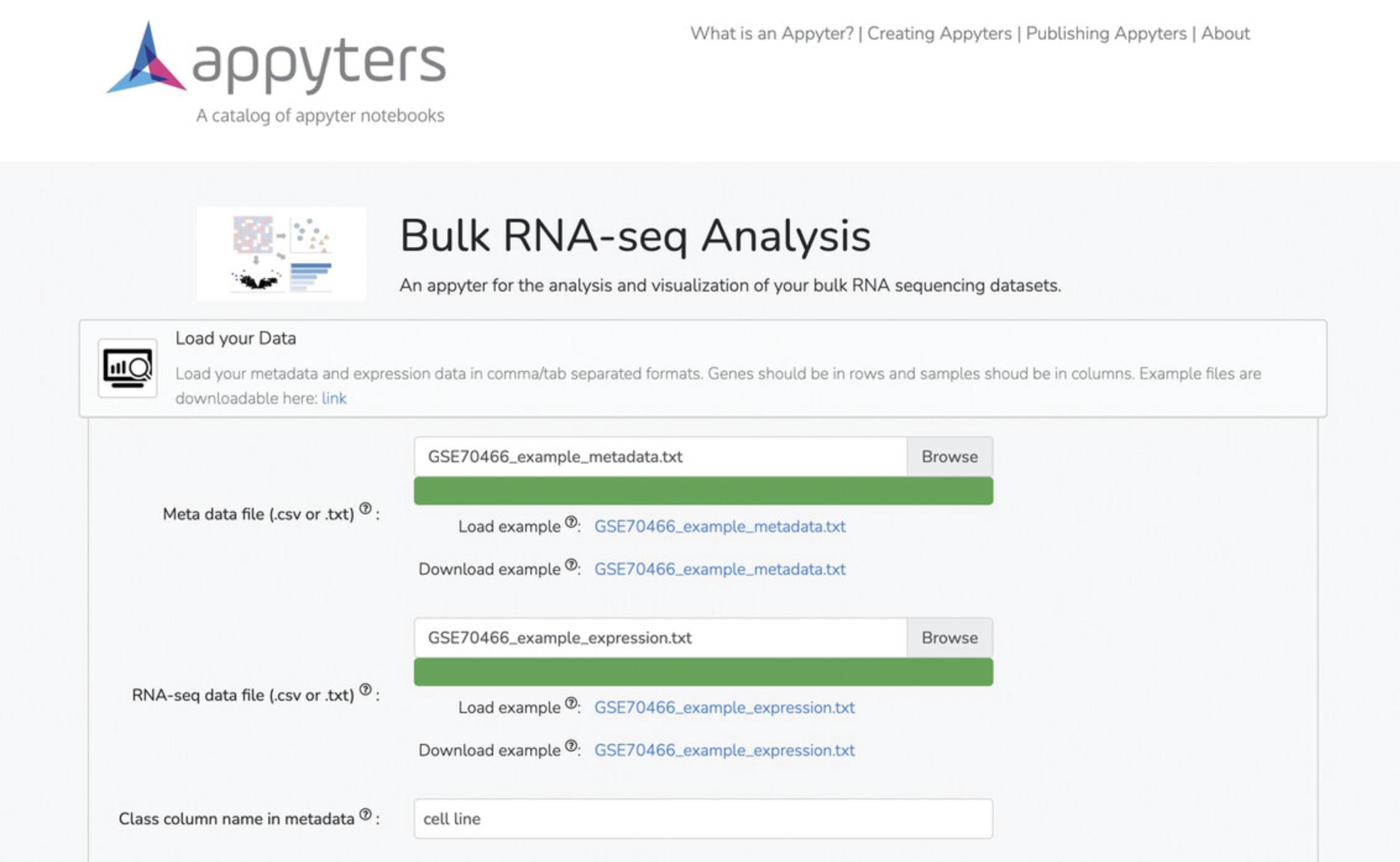
3b. Upload expression data and metadata under the “Load Your Data” tab (Fig. 14).
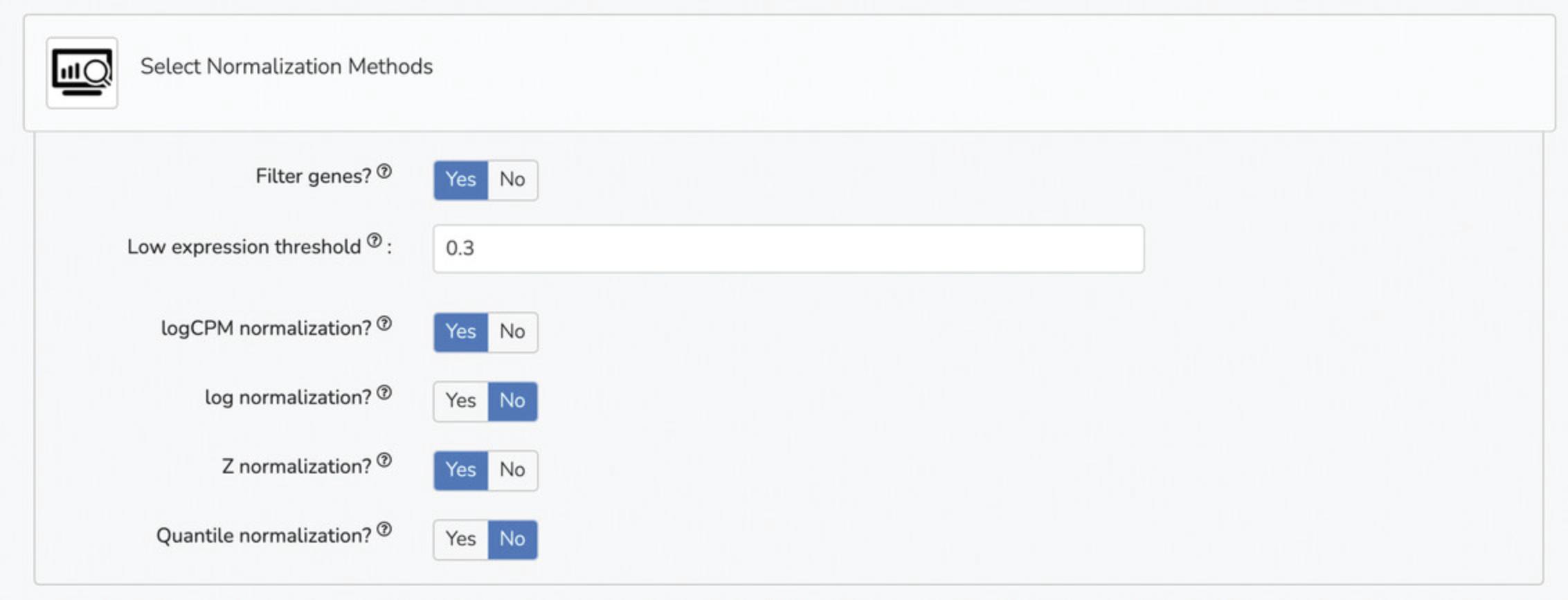
4b. Select the normalization methods under the “Select Normalization Methods” tab. Options include filtering genes , low expression threshold , logCPM normalization , log normalization , Z normalization , and quantile normalization (Fig. 15). Use the default settings if you are unsure about these options.
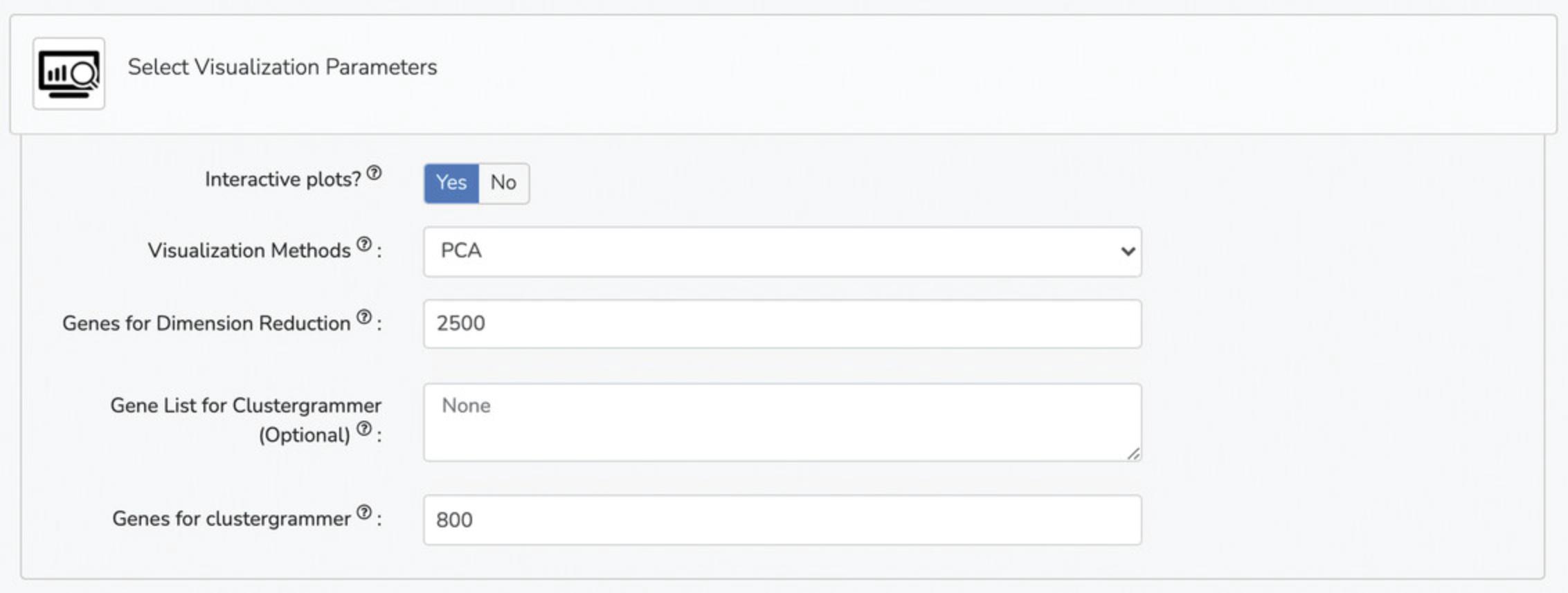
5b. Select visualization parameters under the “Select Visualization Parameters” tab. Options include interactive plots, visualization methods (PCA, UMAP, t-SNE), genes for dimensionality reduction, gene list for Clustergrammer, and genes for Clustergrammer (Fig. 16).
6b. Select differentially expressed gene analysis parameters under the “Select Differentially Expressed Gene Analysis Parameters” tab. Options include differential expression analysis method (limma, characteristic direction, edgeR, DESeq2), differential expression analysis plotting method (volcano plot, MA plot), p-value threshold, logFC threshold, maximum genes for Enrichr, Enrichr libraries (Gene Ontology, Pathway, Kinase, Transcription Factor, and miRNA), top-ranked gene sets, small molecule analysis method (L1000FWD, L1000CDS2), genes for L1000CDS2 or L1000FWD, and top-ranked drugs from L10000CDS2 or L1000FWD (Fig. 17).
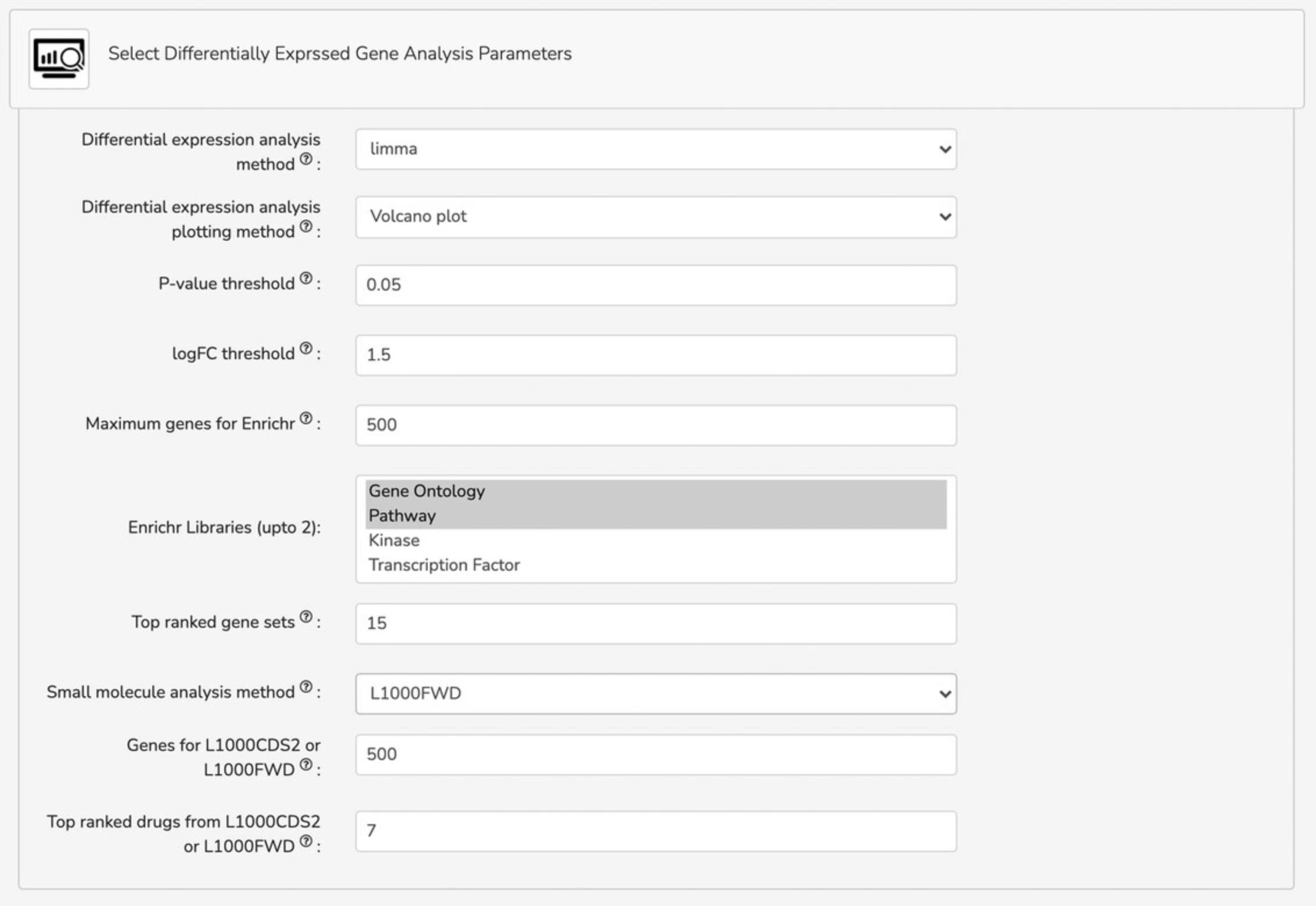
Querying the signatures created from the uploaded data against the L1000 data within the Bulk RNA-seq Appyter
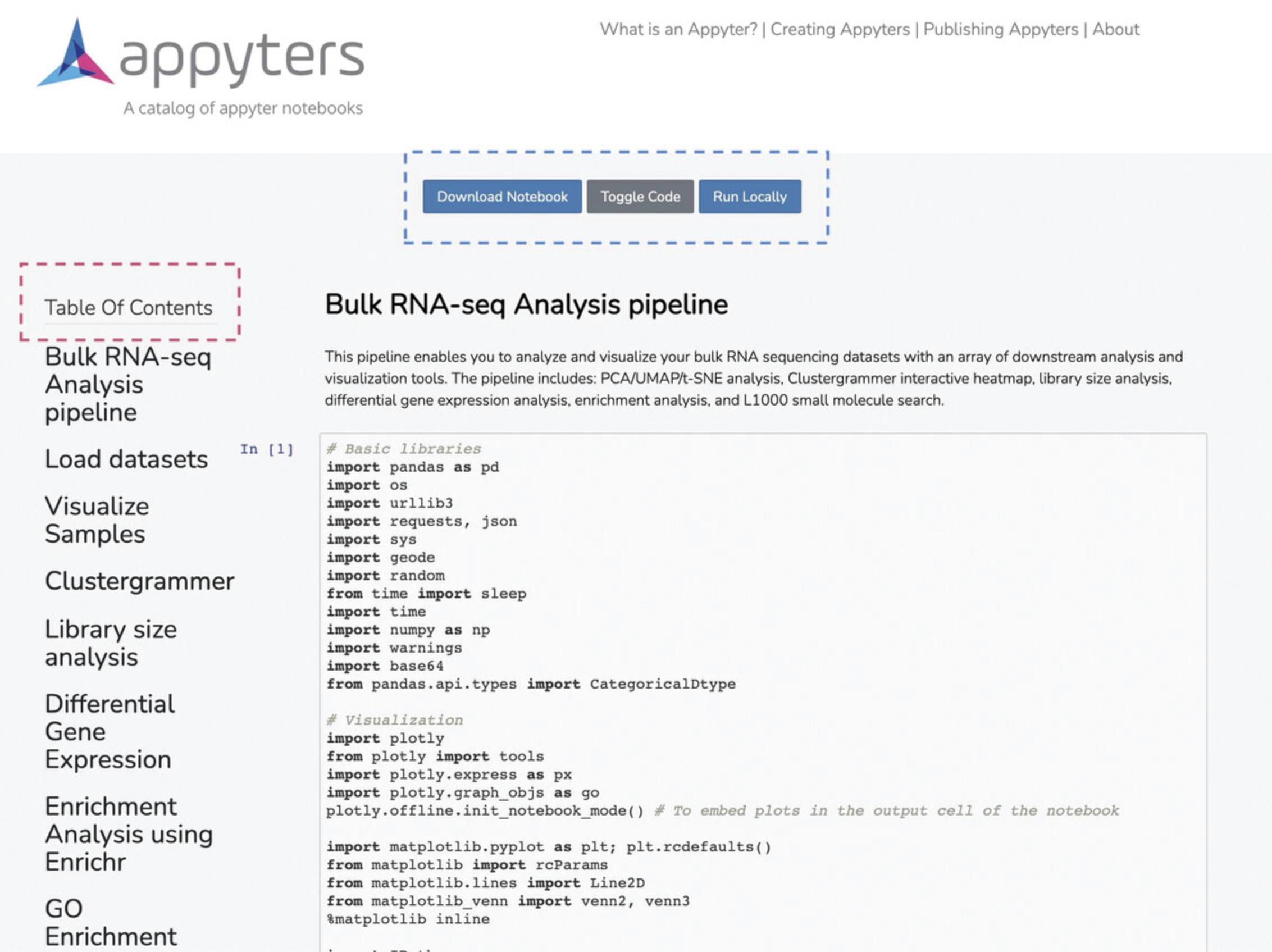
7b. Use the default options and click “Submit” at the bottom of the page to generate your notebook. Once the notebook has loaded, note that there are options to download the notebook, toggle code, and run the notebook locally at the top of the page. The notebook can also be easily navigated using the Table of Contents on the left side of the page (Fig. 18). Use the table of contents to navigate through each analysis section.
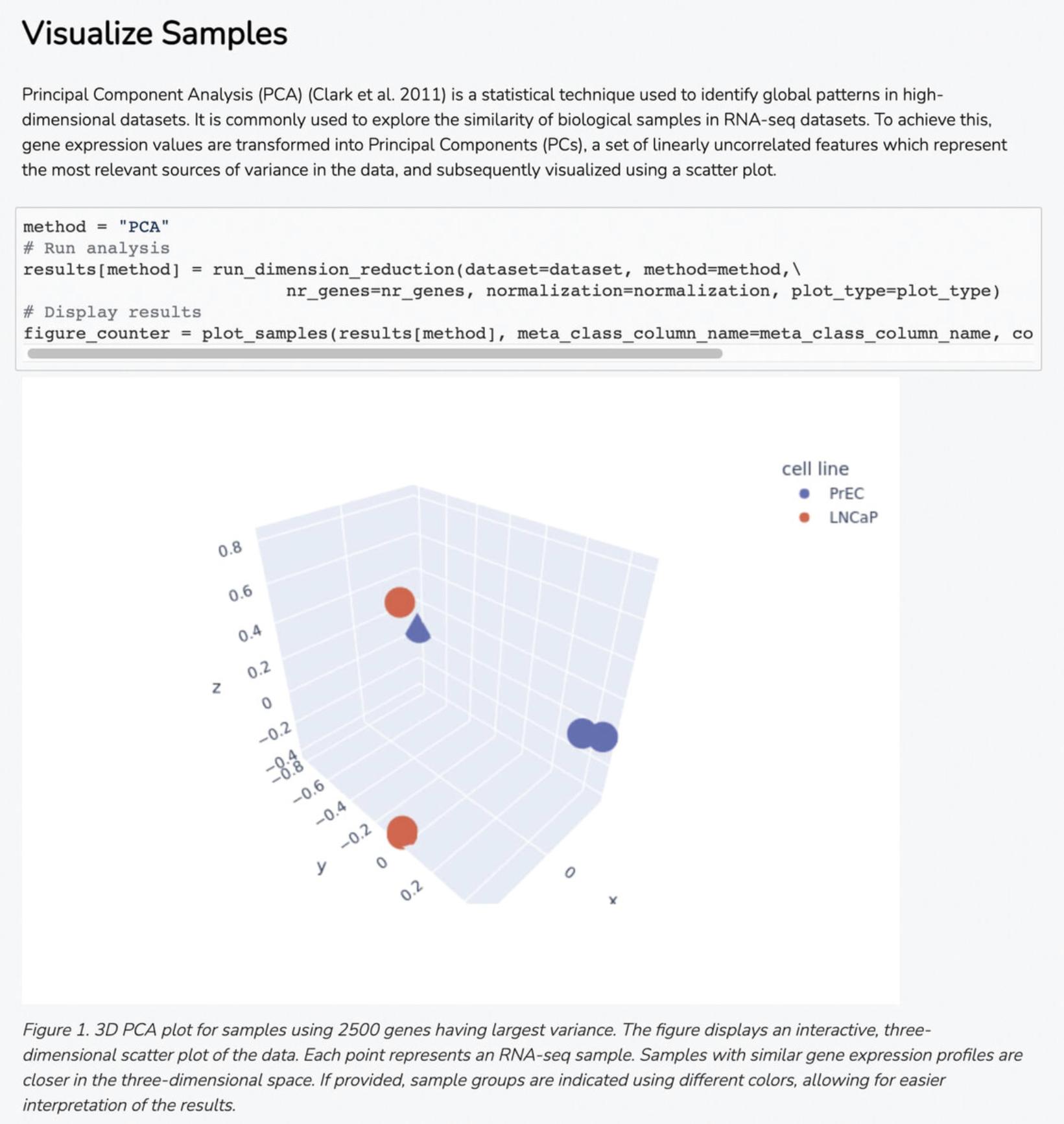
8b. Navigate to the “Visualize Samples” section to view a Principal Component Analysis (PCA) plot made from the 2500 genes with the highest variance in each of the samples, where each of the sample groups are indicated by color (Fig. 19).
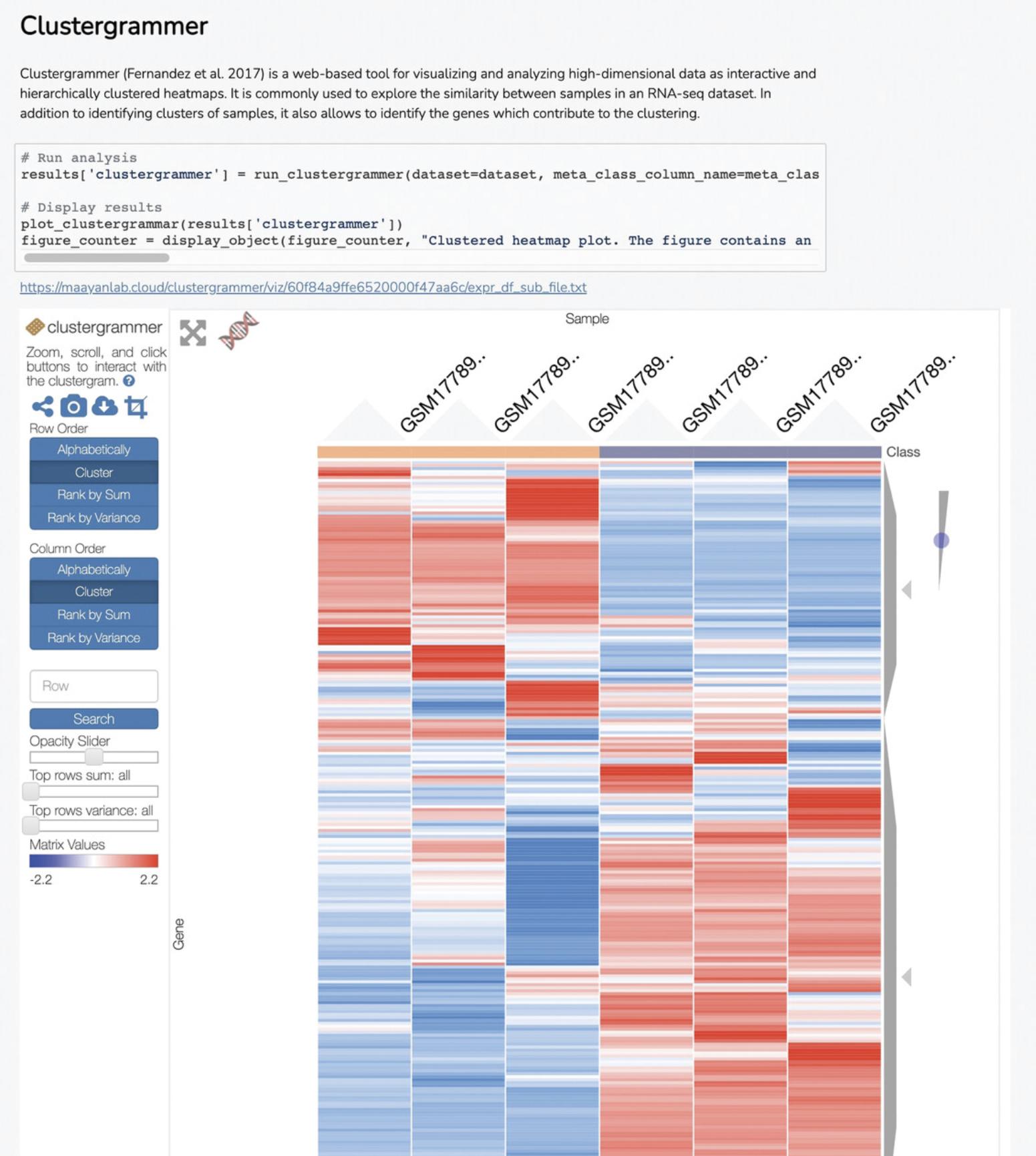
9b. Navigate to the “Clustergrammer” (Fernandez et al., 2017) section to view a heatmap visualization that displays gene expression for each of the genes across all samples, where blue and red indicate decreases or increases in expression, respectively (Fig. 20).
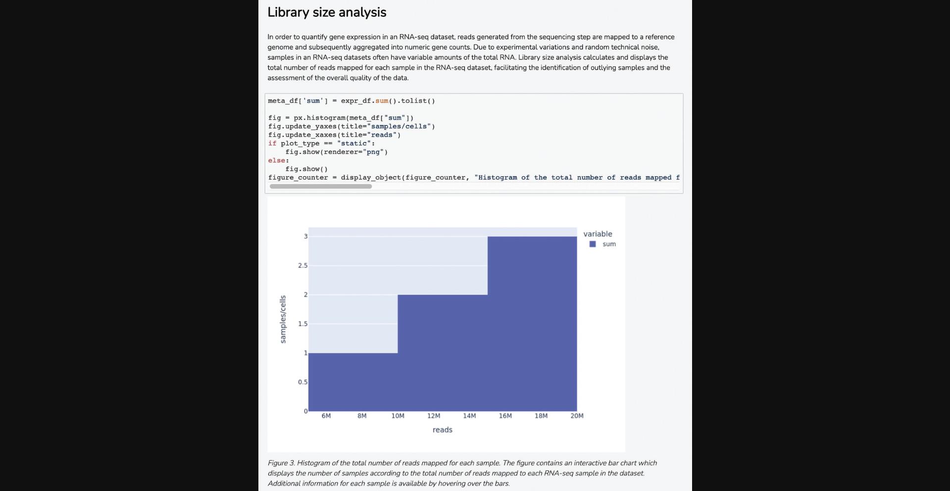
10b. Navigate to the “Library Size Analysis” section to view a histogram that displays the total number of reads matched for each sample, which enables the identification of outlier samples and assesses the overall quality of the RNA-seq data (Fig. 21).
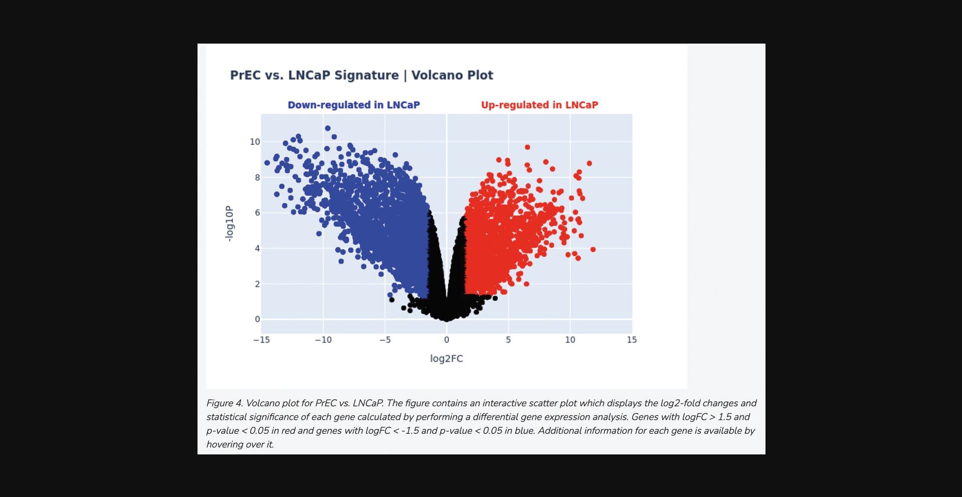
11b. Scroll down to the “Differential Gene Expression” section to view a volcano plot of differential gene expression between the two groups of samples, quantified by log2 fold change and statistical significance of each gene. Blue points correspond to significantly down-regulated genes, whereas red points correspond to significantly up-regulated genes (Fig. 22).
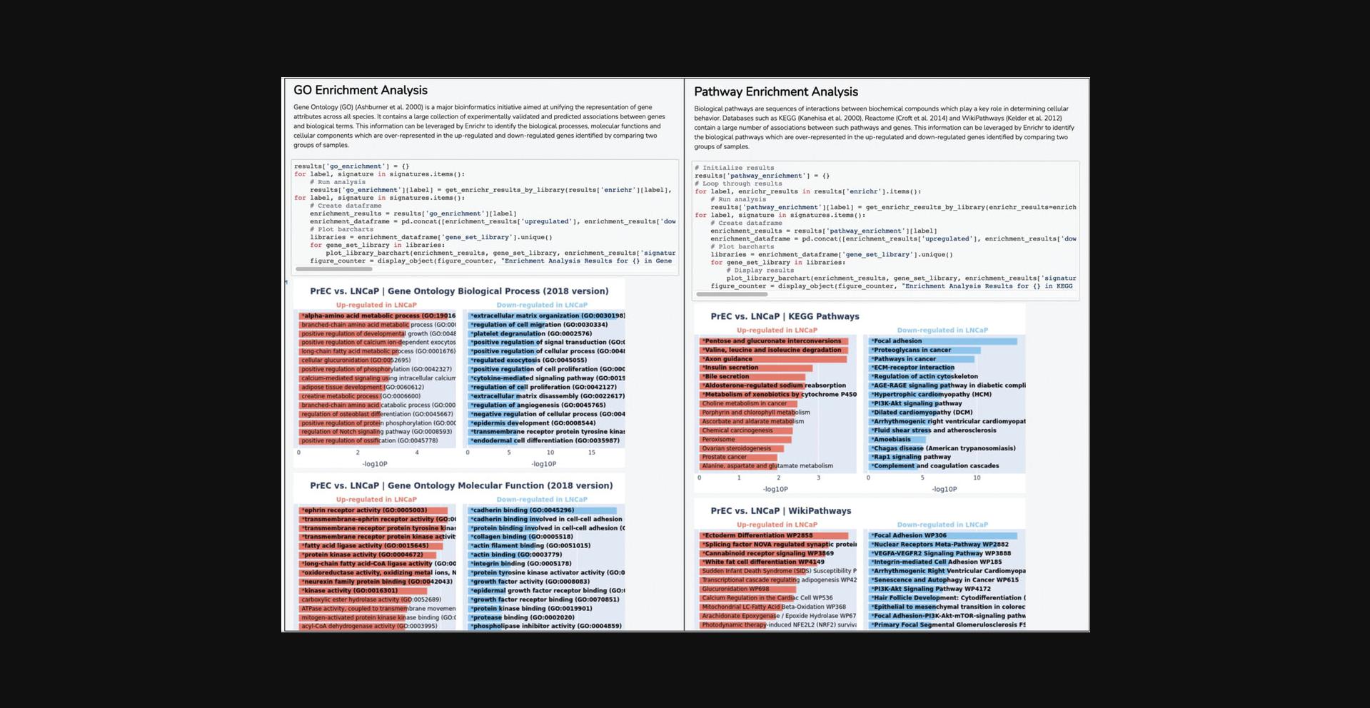
12b. Navigate to the “Enrichment Analysis with Enrichr” section to view bar charts of significantly enriched up and down-regulated terms from the Gene Ontology (The Gene Ontology Consortium, 2019), KEGG (Kanehisa & Goto, 2000), Reactome (Fabregat et al., 2018), and Wikipathways (Kutmon et al., 2016) gene set libraries (Fig. 23).
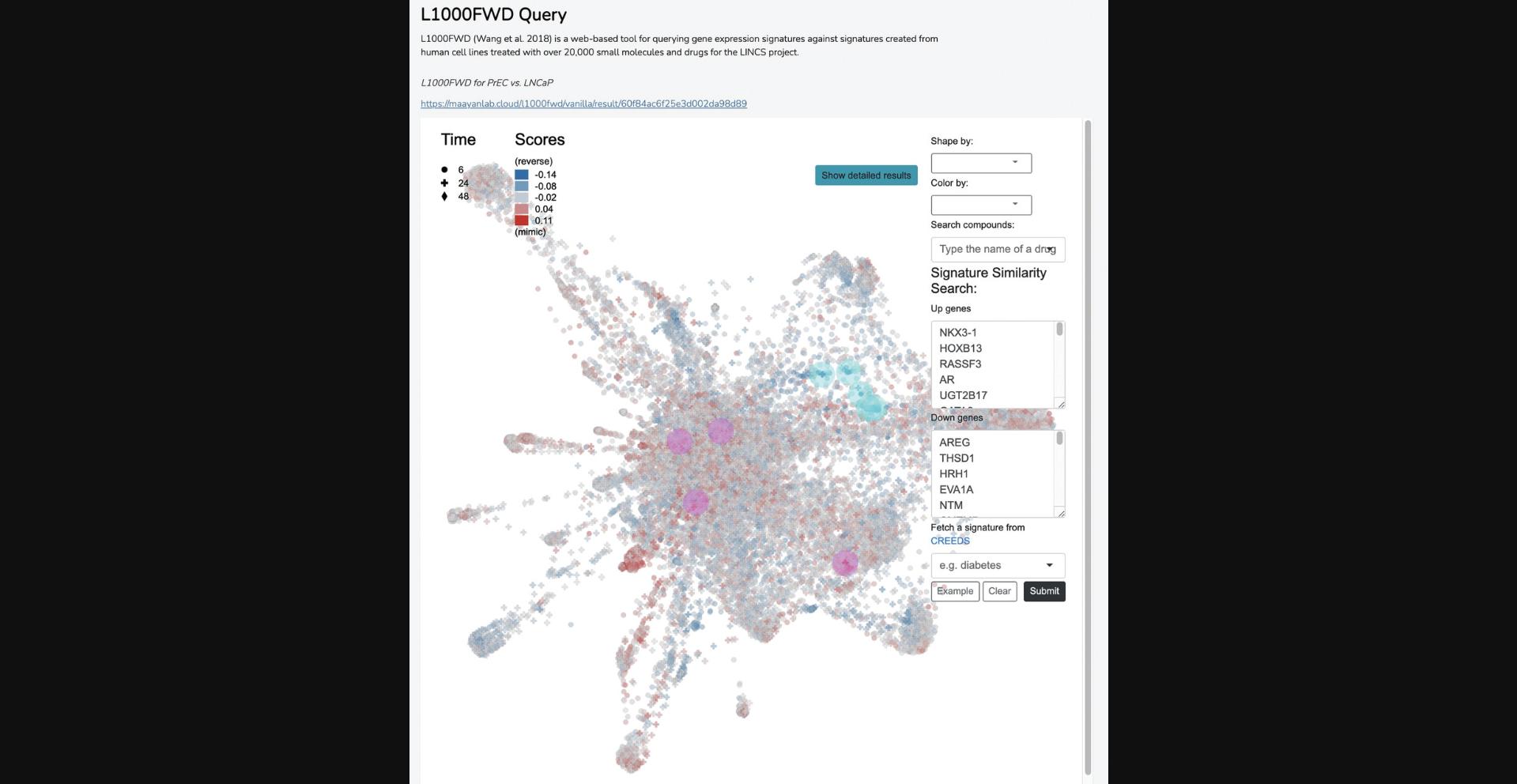
13b. Scroll to the “L1000FWD Query” section to view an interactive display of ∼17,000 L1000 drug-induced gene expression signatures. A downloadable list of mimicking and reversing signatures is provided in the report and available by pressing the blue button on the display. The points on the interactive fireworks display can be shaped and colored by p- value, dose, or time point, and several other options such as MOA, clinical development stage, and automated clustering assignment (Fig. 24).
14b. To save the notebook generated by the Bulk RNA-seq Appyter, click on the blue “Download Notebook” button at the top of the page. The notebook should be downloaded as a Jupyter Notebook (.ipynb) file.
- One way to open an .ipynb file is a console window (e.g., Terminal on MacOS, or Command Prompt on Windows). You may need to install the Jupyter Notebook and iPython packages first. In the console window, navigate to the directory to which the downloaded file was saved (cd
/ /…) and type jupyter notebook to open the notebook in your default web browser.
Basic Protocol 4: UTILIZING THE L1000FWD RESOURCE FOR DRUG DISCOVERY
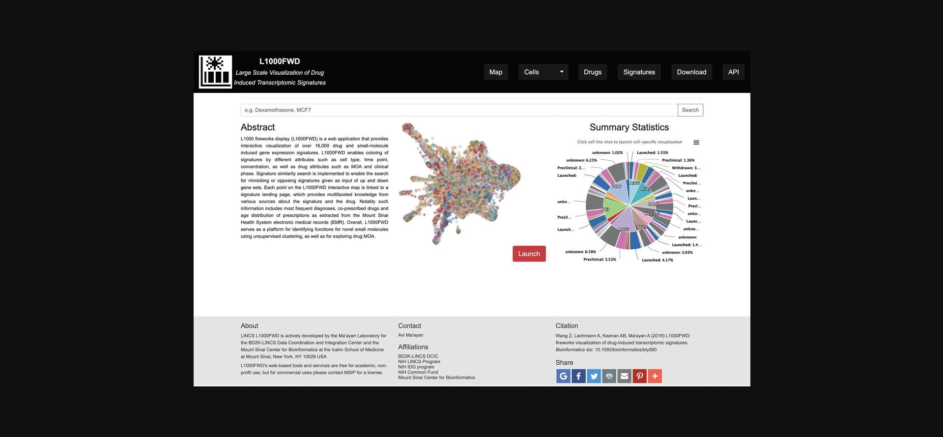
The L1000FWD platform (Wang et al., 2018) provides visualization of drug-induced transcriptomics signatures. The fireworks display is an interactive scatter plot visualizing over 17,000 drug- and small-molecule-induced gene expression signatures as points in two-dimensional space. The L1000FWD map is useful for identifying mechanisms of action (MOA) for novel small molecules using unsupervised clustering, as well as for exploring drugs that may reverse or mimic an input signature of up and down genes. L1000FWD enables coloring of signatures by different attributes including cell type, concentration, and time point, as well as drug attributes including MOA and clinical phase. Each point on the L1000FWD interactive map is linked to a signature landing page, which provides multifaceted knowledge about the signature and the drug from various sources. That information includes most frequent diagnoses, co-prescribed drugs, and patient age distribution of prescriptions extracted from the Mount Sinai electronic medical records (EMR) system.
Necessary Resources
Hardware
Desktop or a laptop computer, or a mobile device, with a fast Internet connection
Software
- An up-to-date web browser such as Google Chrome (https://www.google.com/chrome/), Mozilla Firefox (https://www.mozilla.org/en-US/firefox/), Apple Safari (https://www.apple.com/safari/), or Microsoft Edge (https://www.microsoft.com/en-us/edge)
- Text editor or development environment of choice, such as Visual Studio (https://visualstudio.microsoft.com/vs/)
- Most updated version of Python (https://www.python.org/downloads/) and Python requests library (https://requests.readthedocs.io/en/master/user/install/)
1.Navigate to the L1000FWD homepage (https://maayanlab.cloud/L1000FWD/) (Fig. 25). The homepage includes summary statistics of small molecules profiled in various cell lines, a search bar for querying terms of interest, and a launch button for generating the fireworks visualization.
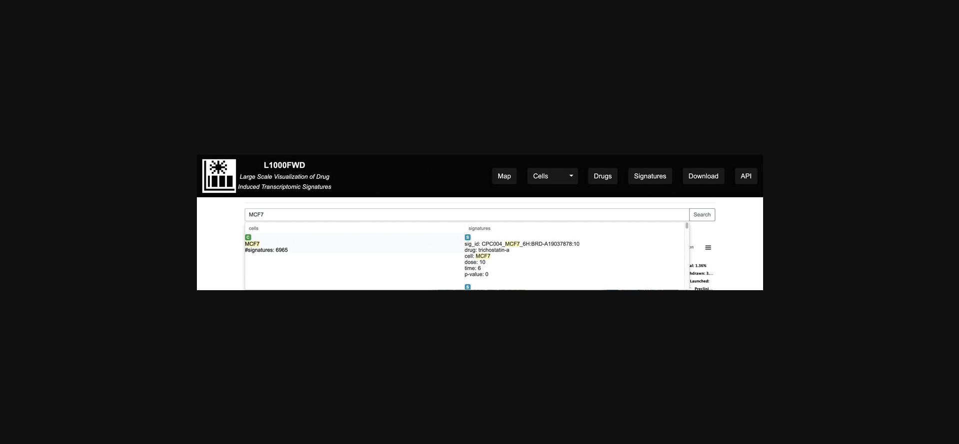
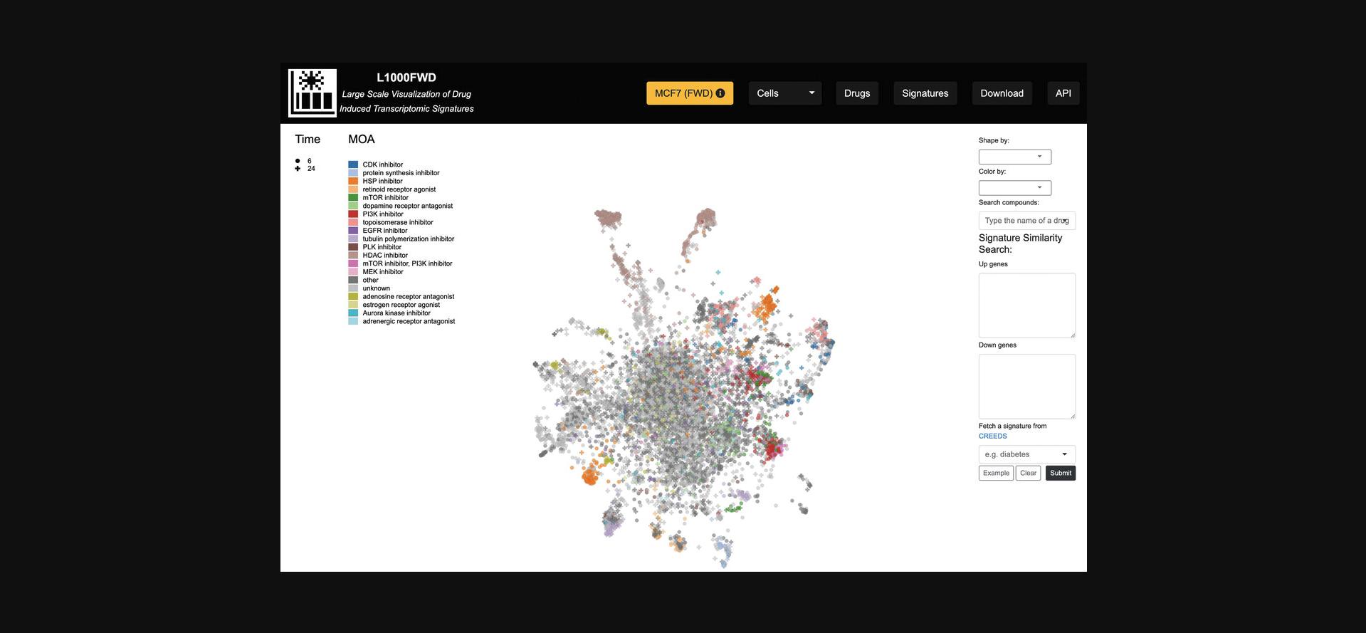
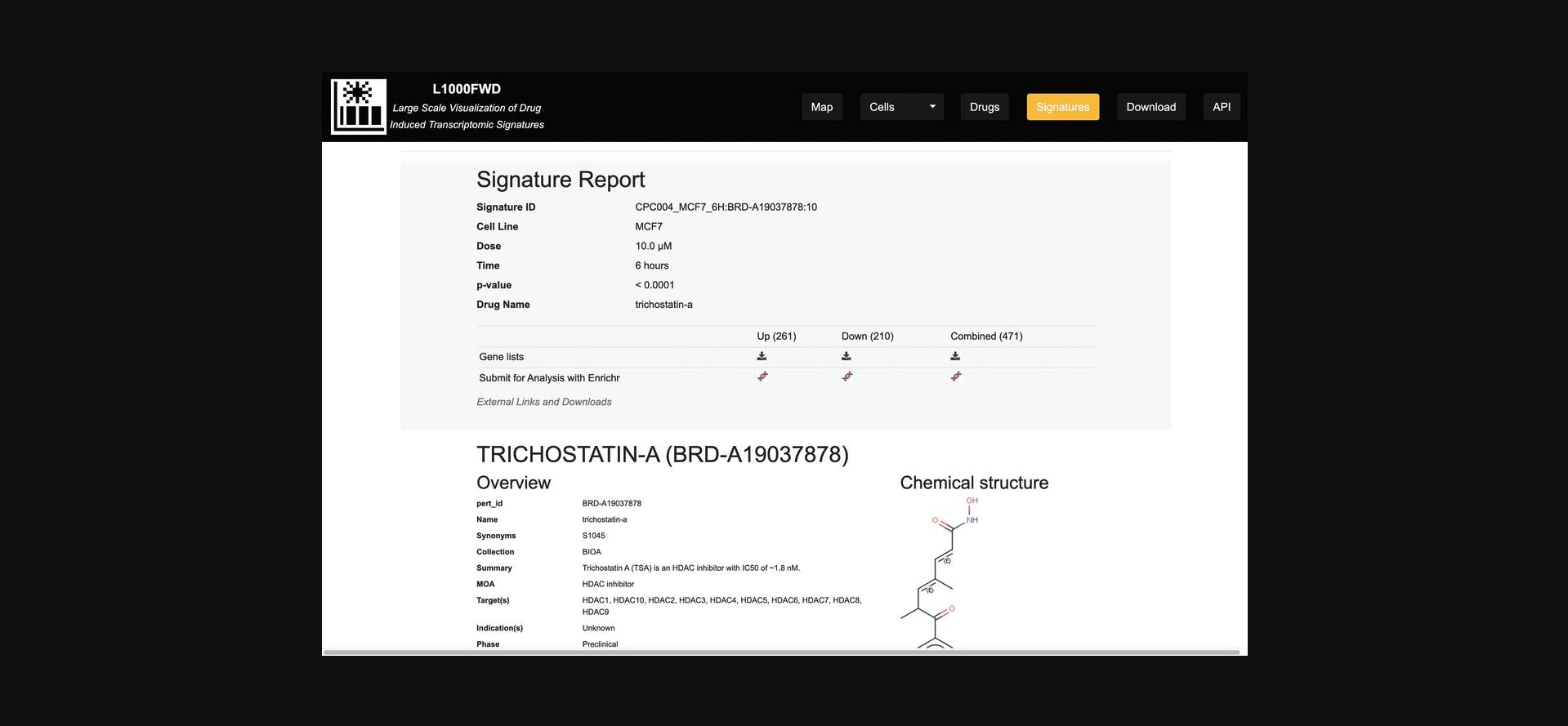
2.On the homepage, type a drug name or cell line query term or phrase of interest in the search field, for example, the cell line MCF7.If a portion of the query string matches an entry in the L1000FWD database, a list of matches will appear as a drop-down (Fig. 26). Clicking on the left element in the drop-down generates a fireworks display filtered by signatures profiled in the MCF7 cell line (Fig. 27), whereas clicking on any of the signatures on the right side of the drop-down menu redirects to a page with identifying metadata for a specific small-molecule signature profiled in the MCF7 cell line (Fig. 28).
Exploring the L1000FWD visualization
3.Click “Launch” on the homepage of L1000FWD to generate the fireworks display with all cell lines, where each of the points represent a drug-induced gene expression signature (Fig. 29). Hovering over a signature displays more information about the signature including the drug name, cell line, concentration, time point, and ID of the signature.
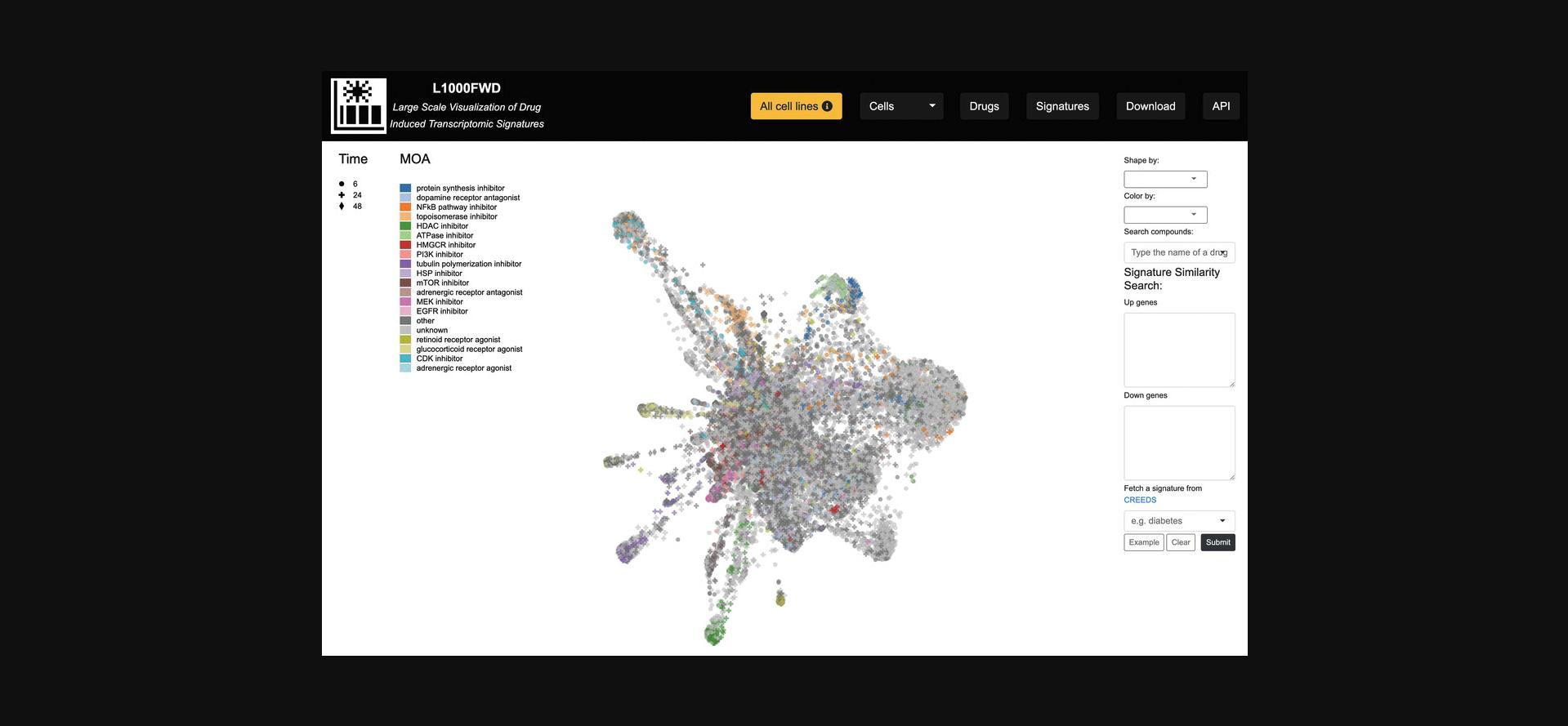
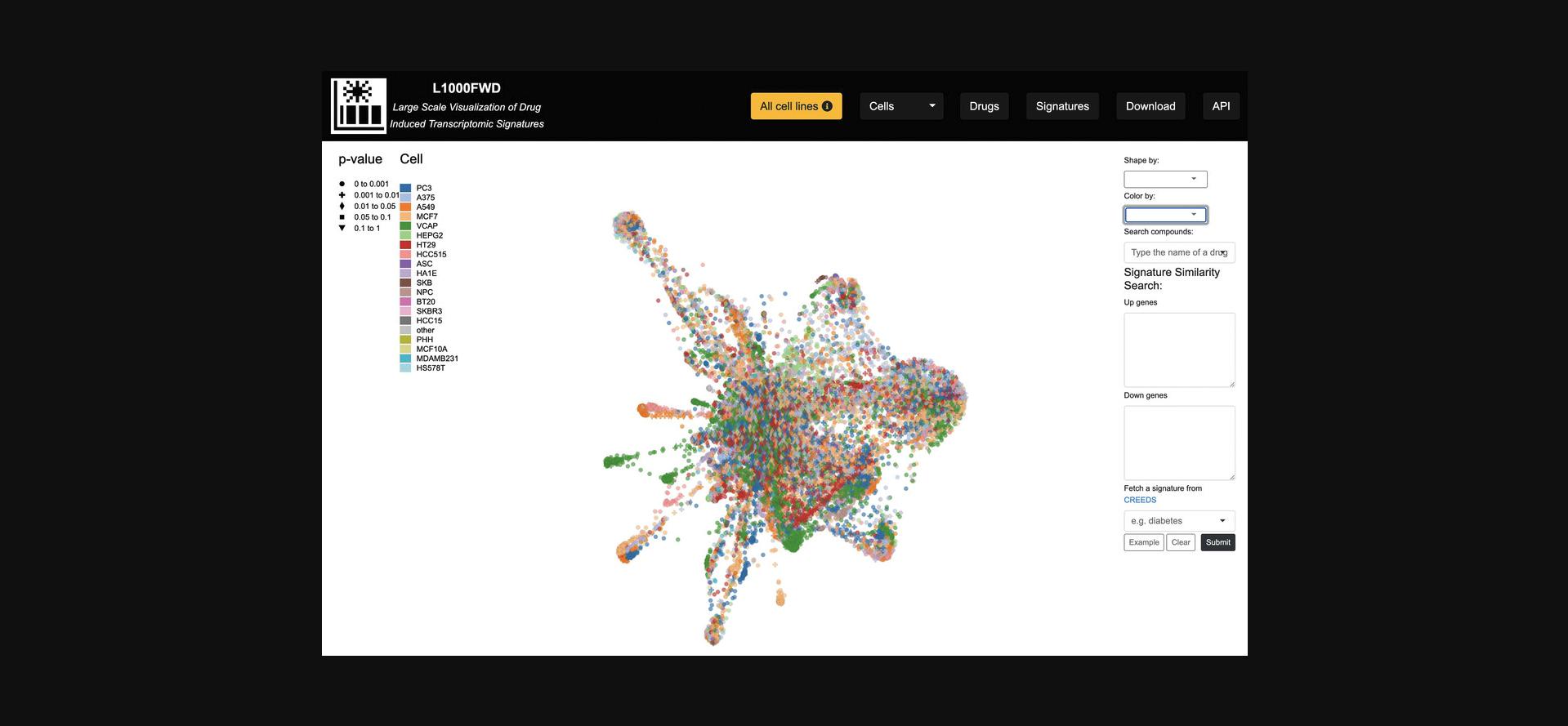
4.There exist several options for altering the visualization, reflected by changes in the shape or color of each signature point. The “Shape by” drop-down menu allows for filtering each signature by p- value, dose, and time points, whereas the “Color by” drop-down menu includes several options for coloring the signatures by cell line, mechanism of action, among several other attributes (Fig. 30).
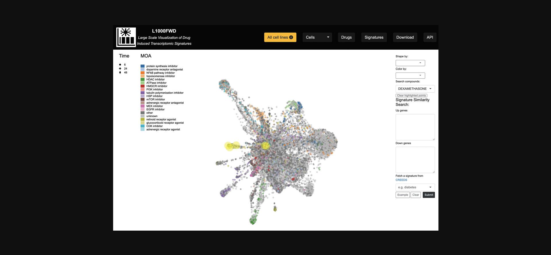
5.The “Search compounds” autocomplete textbox enables the input of a small molecule whose signatures will be highlighted in the visualization (Fig. 31).
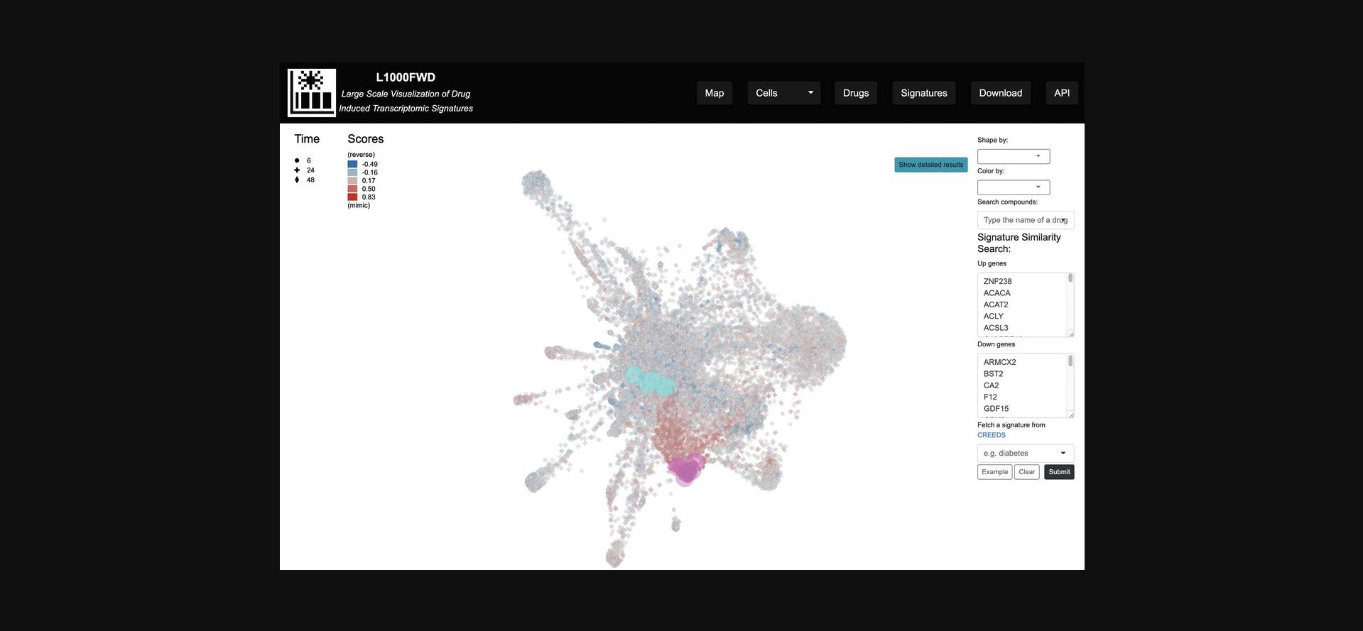
6.In the “Signature Similarity Search” section to the right of the plot, enter a list of up-regulated genes and a list of down-regulated genes, and click the Submit button. The gene lists can be pre-populated with example data by clicking the “Example” button. Regions in the gene expression space that mimic or reverse the submitted up/down genes will be highlighted in red and blue, respectively (Fig. 32). Alternatively, a signature including up/down genes from CREEDS (Wang et al., 2016) can be submitted by inputting a query term in the autocomplete field.
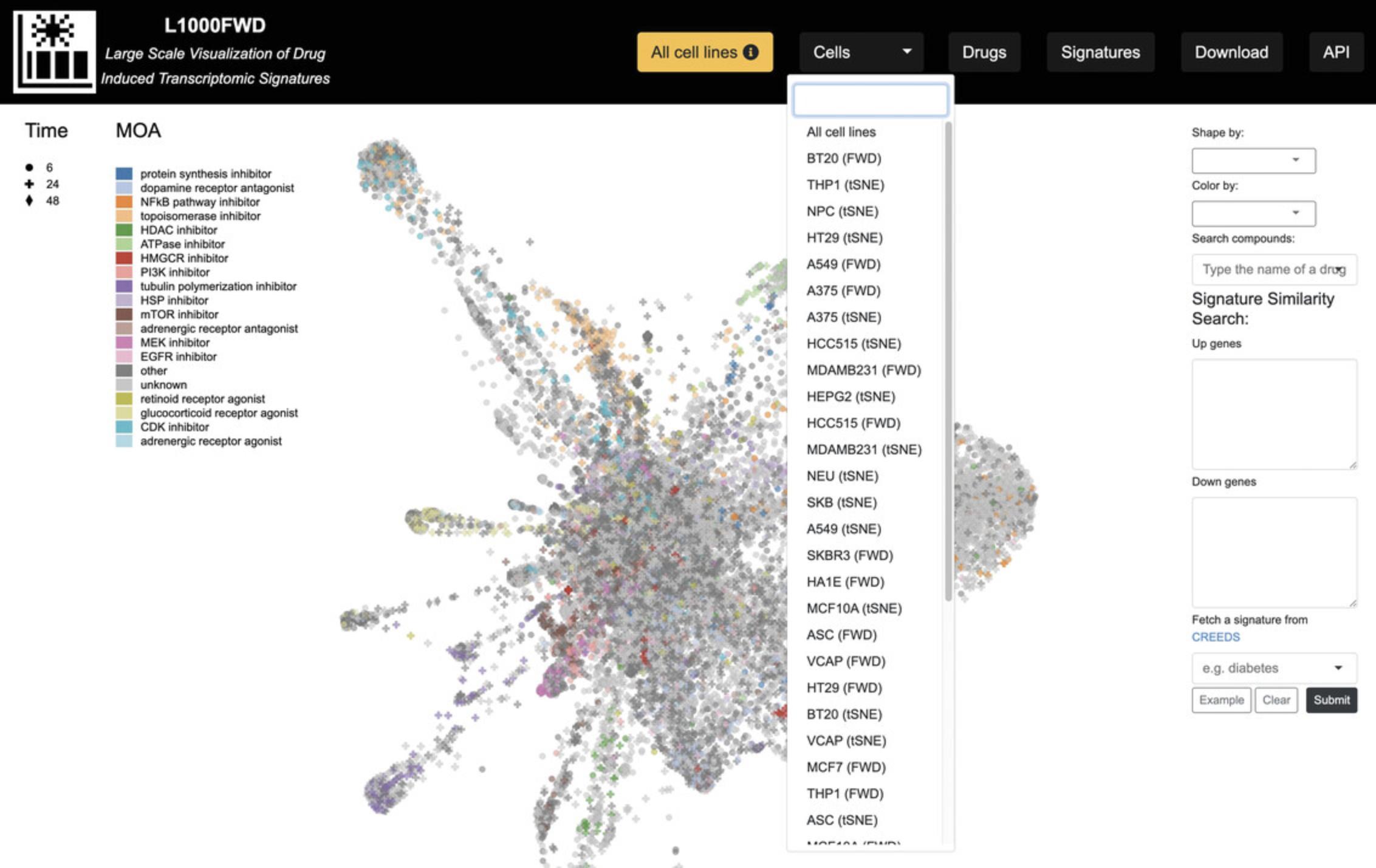
7.By default, signatures profiled in all cell lines are included. In the navigation bar at the top of the page, click the “Cells” drop-down menu and select a cell line of interest to filter the resulting visualizations by signatures that were only profiled in the selected cell line (Fig. 33).
Viewing collections of signature reports for an individual drug
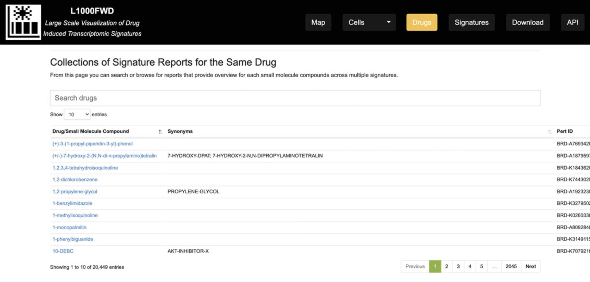
8.On the homepage, click the “Drugs” button on the top menu. You will be navigated to a table listing 20,000+ drugs (Fig. 34); this table can be browsed as well as manually searched using the “Search drugs” panel. For each drug, a hyperlinked landing page is provided to list properties of the drug including name, LINCS perturbagen ID, MOAs, and target(s), if known, and chemical and structural properties. For drugs that have associated L1000 signatures, a table with title “Gene signatures” is provided on the drug's landing page; for each entry, the table lists the Signature ID, p- value, cell type, and dose.
Generating signature reports
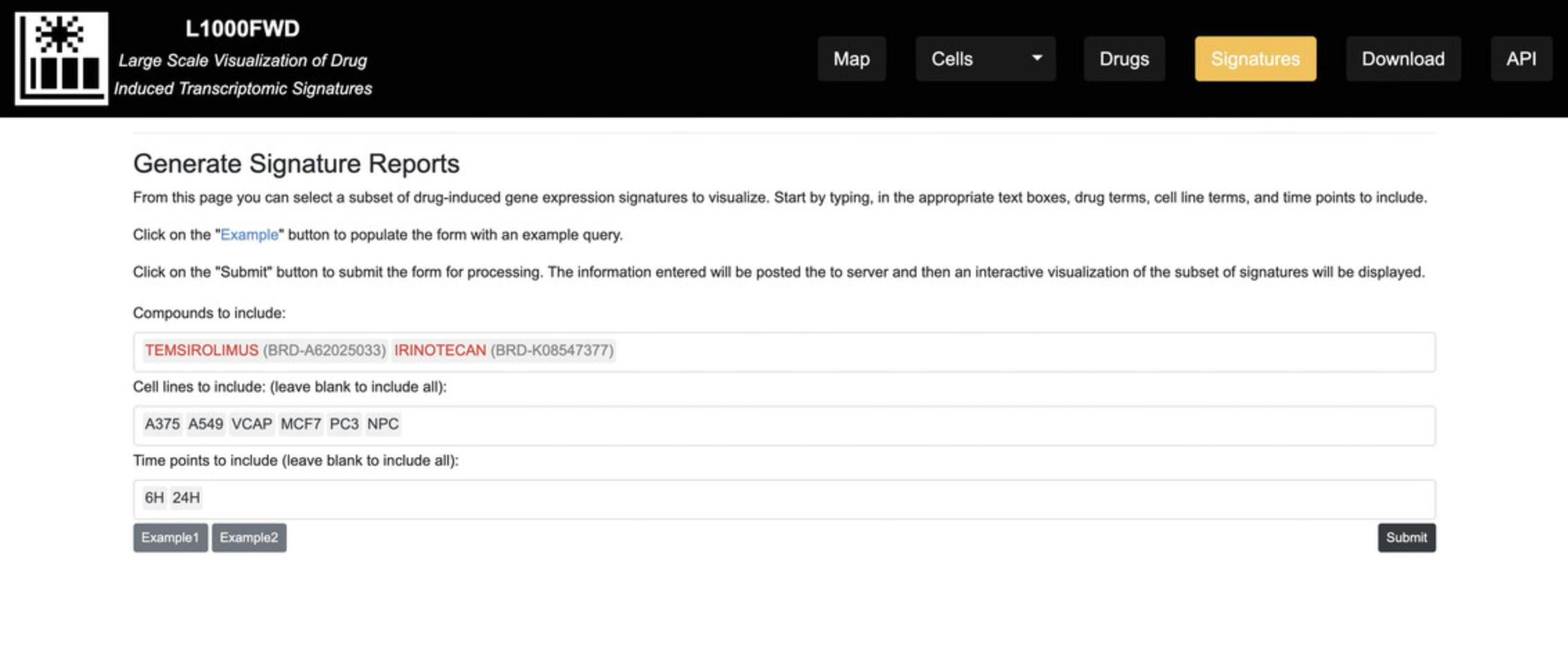
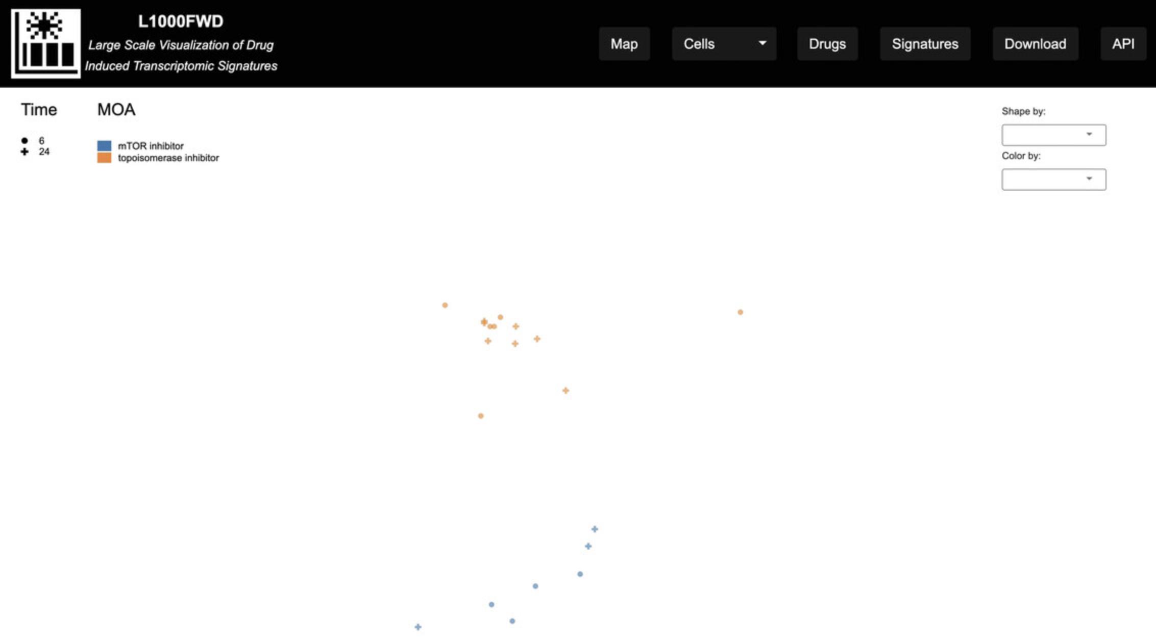
9.On the homepage, click on the “Signatures” button on the top menu. You will be navigated to the Generate Signature Reports page (Fig. 35), which facilitates selecting a subset of drug-induced gene expression signatures to visualize. Click “Example 1” to populate the fields with compounds, cell lines, and time points to filter a subset of signatures. Click on the “Submit” button to submit the form for processing. The information entered will be posted to the server, and an interactive visualization of the subset of signatures will be displayed (Fig. 36).
Downloading L1000FWD data
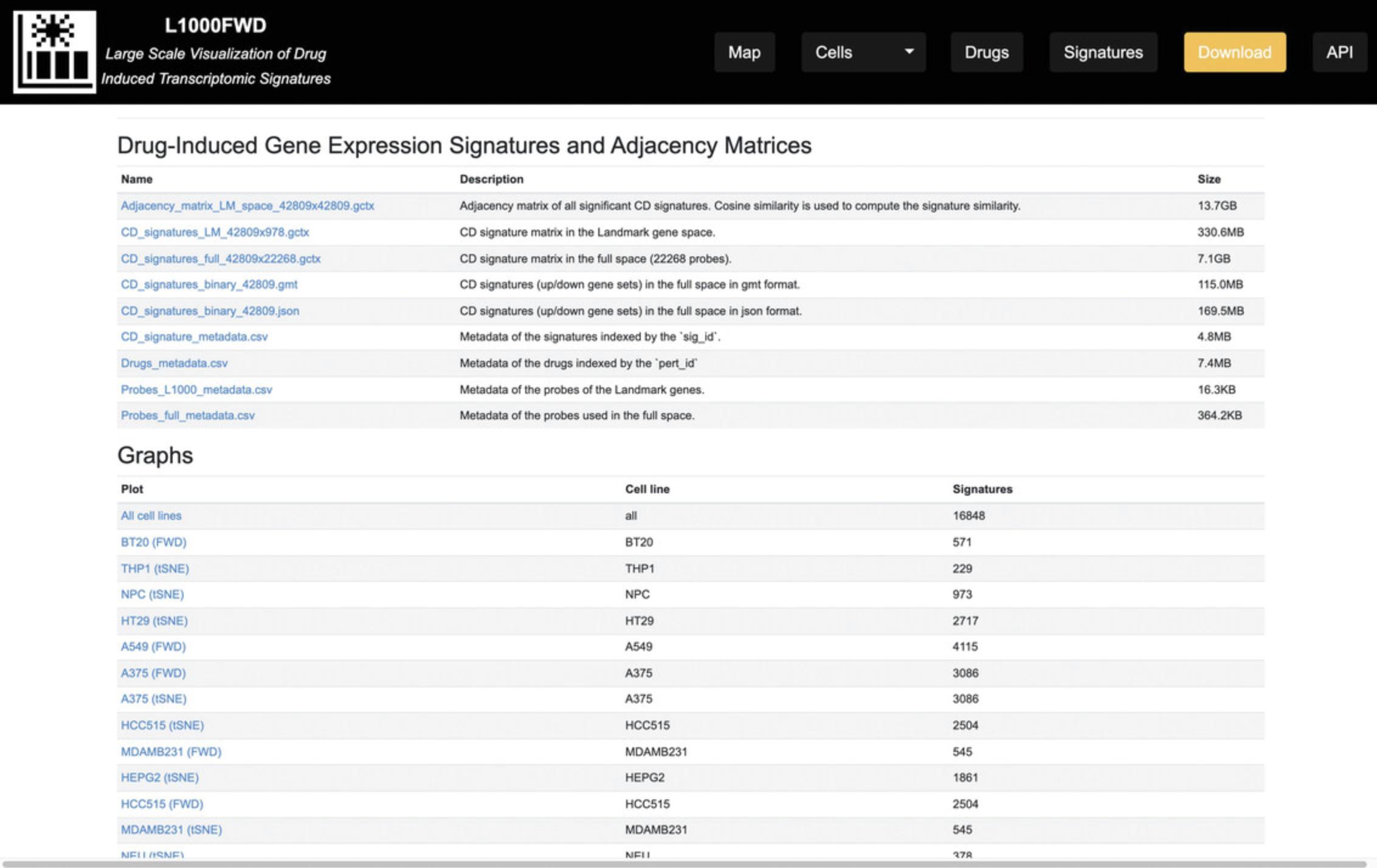
10.On the homepage, click on the “Download” button on the top menu; you will be navigated to the Downloads page (Fig. 37), which includes two sections of content: Drug-Induced Gene Expression Signatures and Adjacency Matrices and Graphs.
-
Download Content from the Drug-Induced Gene Expression Signatures and Adjacency Matrices Section: this table lists the filenames, and associated file descriptions and sizes. The files in this table have various formats, including GCTX, GMT, JSON, and CSV. For any of the nine entries listed in this table, click on the entry's hyperlink in the left column of the table to download each file.
-
Download Content from Graphs Section: this section provides the datasets associated with the All Cells L1000FWD plot and the 40 L1000 and t-SNE plots for individual cell lines. The associated cell line and number of signatures are listed in the table. Click on the hyperlink in the left column for any entry to download its dataset.
Using the L1000FWD API
11.Open a new or existing Python code file. Import the “JSON” and “requests” libraries at the top of the file as follows.
- import json
- import requests
12.Call the requests.get method to send a GET request to the URL. The query_string variable contains the string that is sent to the L1000FWD_URL/synonyms endpoint. If the endpoint is available, then the response is saved to a JSON file.
- L1000FWD_URL = 'ht tps://maayanlab.cloud/L1000FWD/'
- query_string = 'dex'
- response = requests.get(L1000FWD_URL + 'synonyms/' + query_string)
- if response.status_code == 200:
- pprint(response.json())
- json.dump(response.json(), open('api1_result.json', 'wb'), indent=4)
13.View the response as a JSON object containing all drug objects that match the query string.
- [
- {
- "pert_id": "BRD-K07265709",
- "Name": "DEXRAZOXANE"
- },
- {
- "pert_id": "BRD-A93424738",
- "Name": "DEXAMETHASONE-ACETATE"
- },
- {
- "pert_id": "BRD-A10188456",
- "Name": "DEXAMETHASONE"
- },
- {
- …
- ]
For more information on using the various L1000FWD API endpoints, please refer to the API documentation (https://maayanlab.cloud/L1000FWD/api_page).
Basic Protocol 5: KINOMEscan AND THE KINOMEscan APPYTER
KINOMEscan is a commercial kinase profiling assay provided by DiscoveRx. The KINOMEscan assay is based on competitive binding, in which each drug or compound of interest is run against a panel of approximately 440 purified kinases. Results are reported as “percent of control” (% control), which represent the amount of kinase-ligand binding observed when a test compound is present, compared to the control compound DMSO. As part of the LINCS program, the Harvard Medical School (HMS) LINCS DSGC profiled ∼180 different drugs and small molecules with KINOMEscan (Fabian et al., 2005). The KINOMEscan Data Visualization Appyter (https://appyters.maayanlab.cloud/#/KINOMEscan) provides tables and bar chart visualizations of KINOMEscan data for kinase and small molecule queries. The Appyter can also identify drug targets and perform kinase enrichment analysis based on an input protein set.
Necessary Resources
Hardware
Desktop or a laptop computer, or a mobile device, with a fast Internet connection
Software
- An up-to-date web browser such as Google Chrome (https://www.google.com/chrome/), Mozilla Firefox (https://www.mozilla.org/en-US/firefox/), Apple Safari (https://www.apple.com/safari/), or Microsoft Edge (https://www.microsoft.com/en-us/edge)
Accessing KINOMEscan data
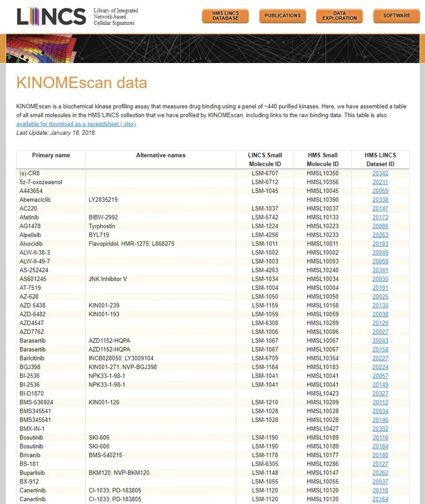
1.Navigate to the KINOMEscan section of the HMS LINCS Database (https://lincs.hms.harvard.edu/kinomescan/). The table on this page displays information on all small molecules profiled by the HMS LINCS Center, including each molecule's primary name, alternative names, LINCS Small Molecule ID, HMS Small Molecule ID, and corresponding HMS LINCS Dataset ID (Fig. 38). To download the entire table as an Excel spreadsheet, click the “available for download as a spreadsheet (.xlsx)” link in the explanatory paragraph. For multiple downloads, right click the link, select “Save link as…” and save the spreadsheet to the desired local folder.
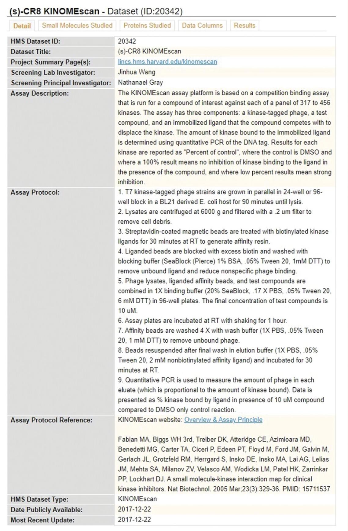
2.Click on any ID in the “HMS LINCS Dataset ID” column to view a specific dataset. By default, the “Detail” tab is shown on the new page, which provides project information, assay metadata, and other information relevant to the specific profiling assay (Fig. 39).
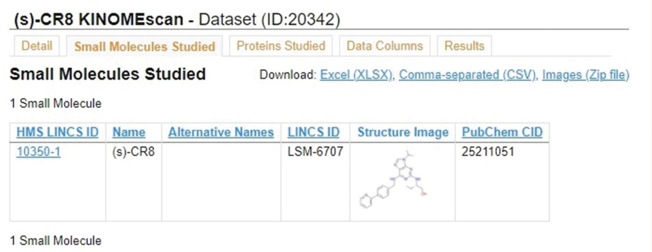
3.Click the “Small Molecules Studied” tab (Fig. 40) to view metadata on the small molecule profiled in this dataset, including the structural image and PubChem ID of the molecule.
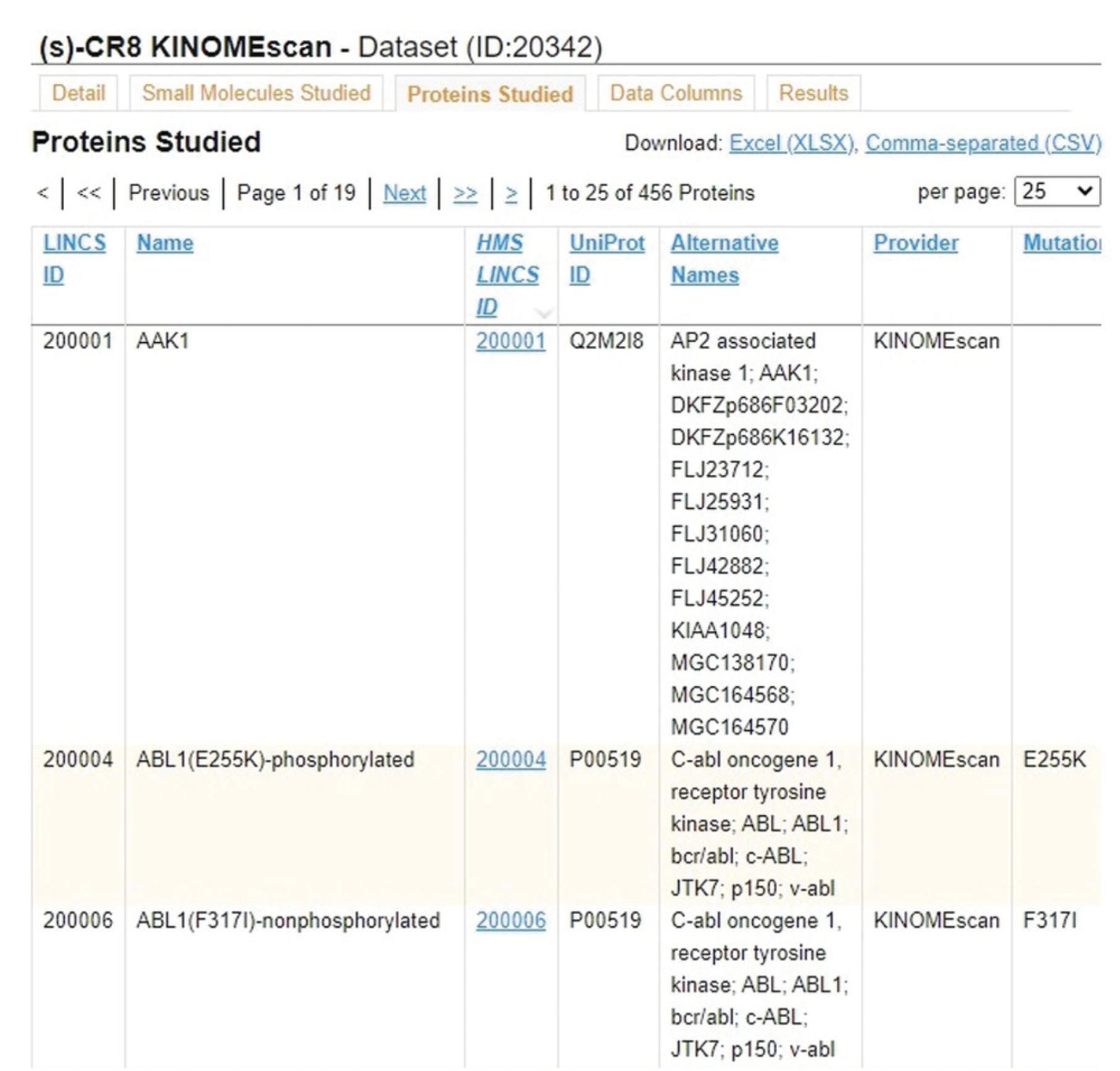
4.Click the “Proteins Studied” tab (Fig. 41) to view metadata on all panel kinases used in this dataset, including identifiers, names, domain, mutations, and phosphorylation states.
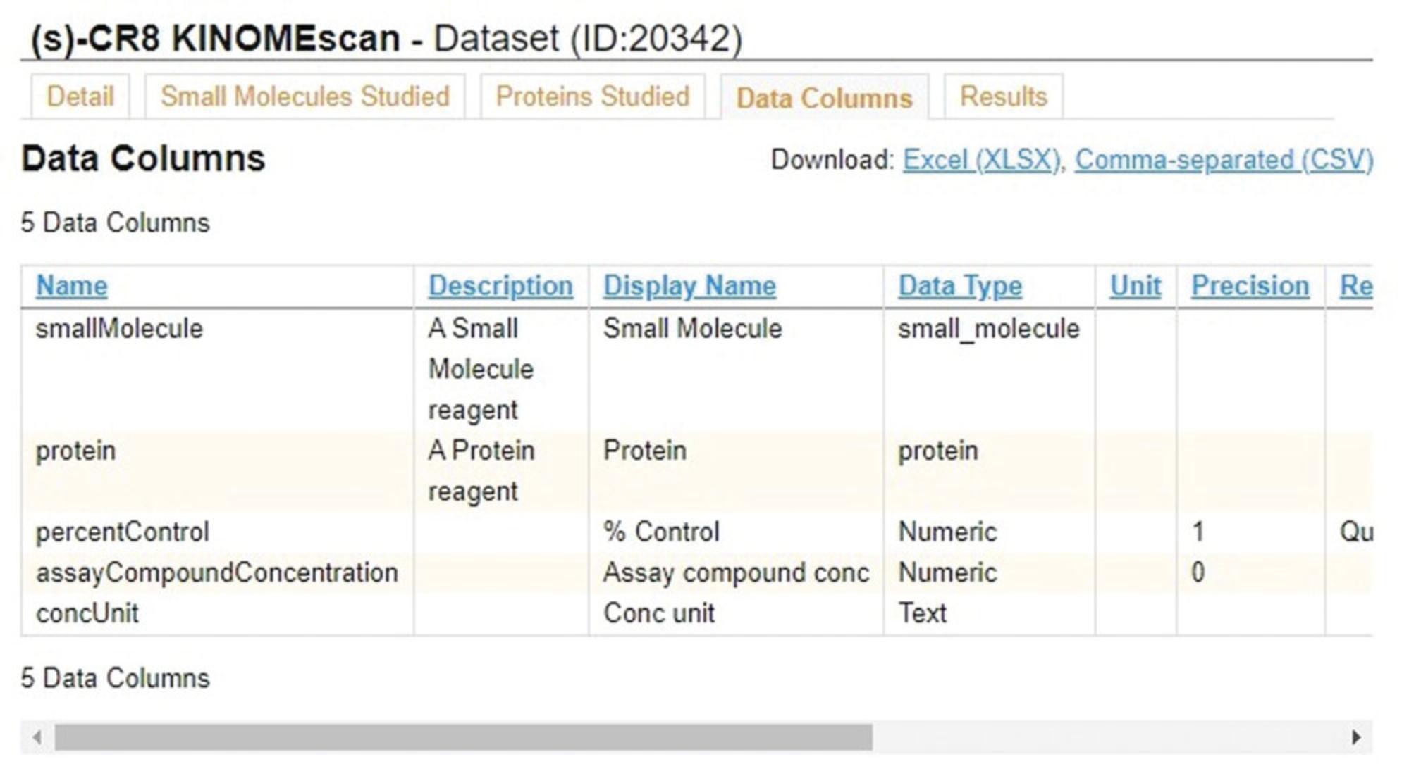
5.Click the “Data Columns” tab (Fig. 42) to view metadata and descriptions for each of the columns in the results table for the given dataset.
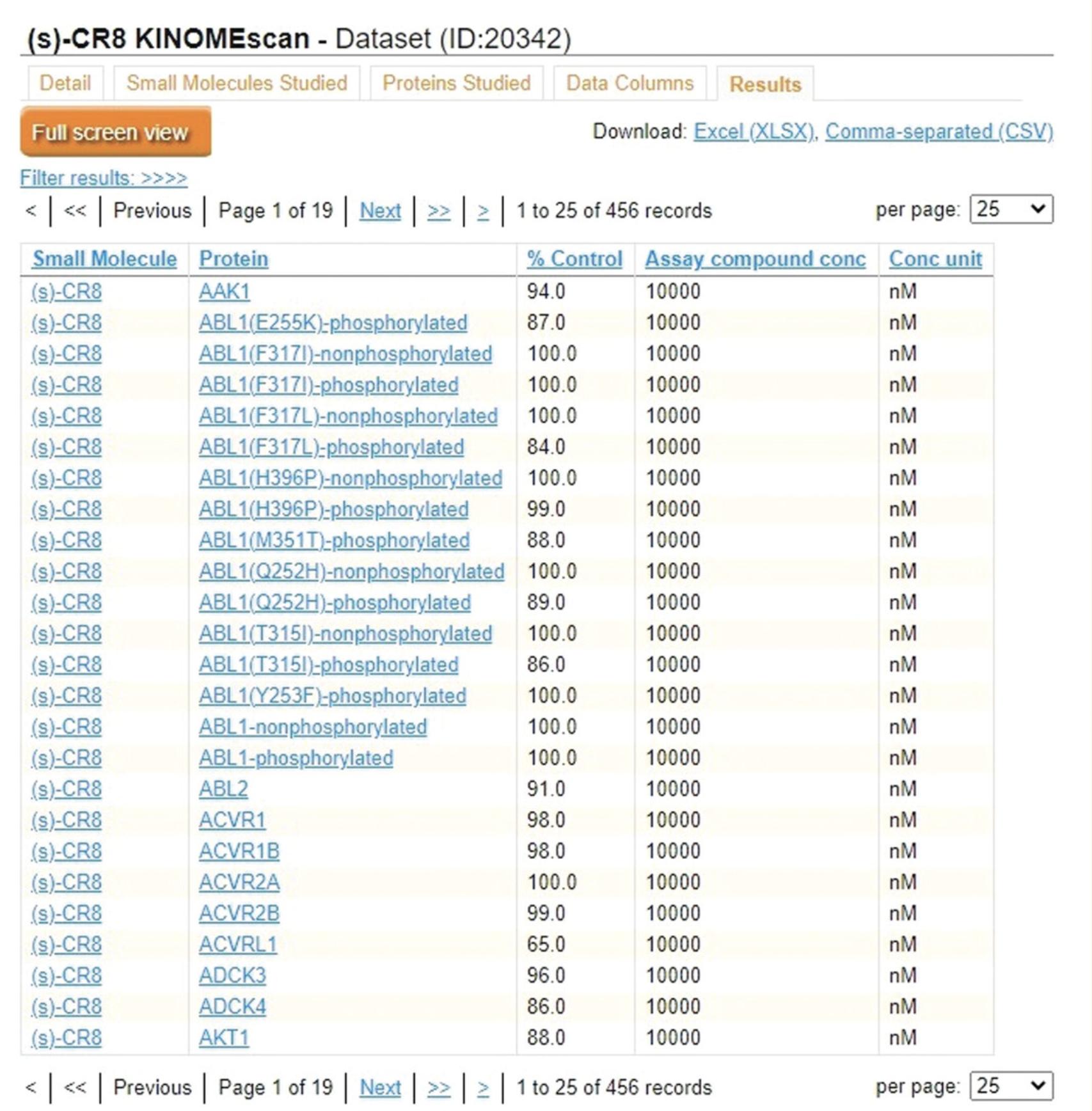
6.Click the “Results” tab (Fig. 43) to view the results of the assay. The % control and equilibrium dissociation constant (Kd) quantify binding of the corresponding protein kinase in each row to a ligand when the tested small molecule was present.
7.Use the download links in the top right corner of any tab to download the full table on that tab as either an Excel (.xlsx) or CSV file.
Querying a kinase with the KINOMEscan Data Visualization Appyter
8.Navigate to the KINOMEscan Data Visualization Appyter at https://appyters.maayanlab.cloud/#/KINOMEscan and click the “Start Appyter” button to view the input form (Fig. 44).
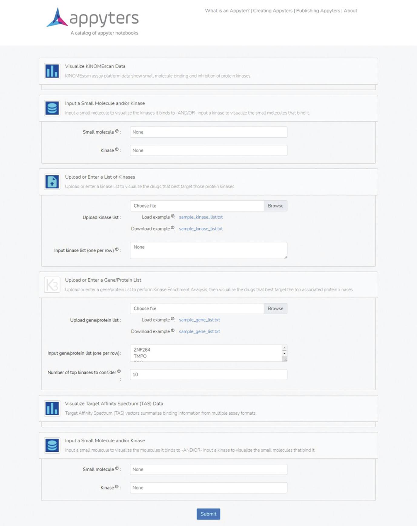
9.Under the section heading “Input a Small Molecule and/or Kinase”, enter a kinase of interest into the “Kinase” search box. Scroll to the bottom of the input form and click the blue “Submit” button.
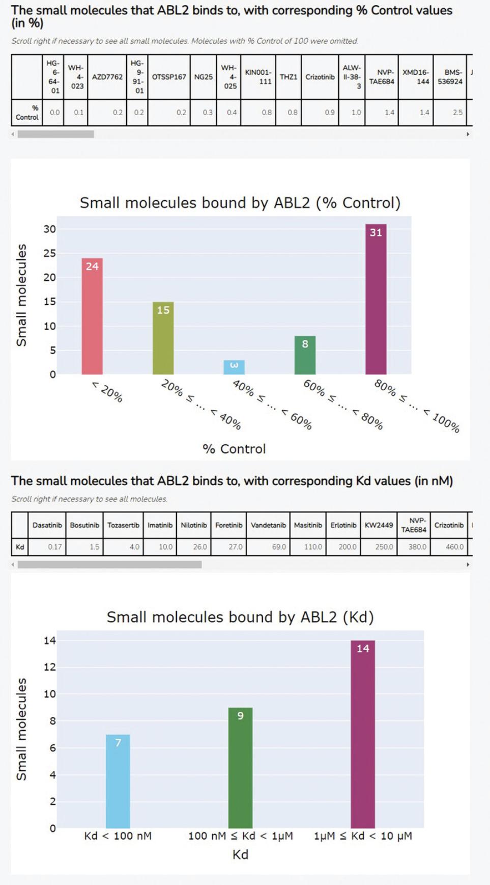
10.The Appyter will automatically begin execution. When execution has completed, as indicated by the “Success” box at the top of the page, scroll down to the section titled “Generate table and bar chart of small molecules for kinase input from KINOMEscan data” to view the results (Fig. 45). The tables show the top-ranked small molecules that bind the input kinase, based on both % control and Kd values; the bar charts show the distribution of % control and Kd values among all small molecules which bind the input kinase.
Querying a small molecule in the KINOMEscan Data Visualization Appyter
11.Navigate to the KINOMEscan Data Visualization Appyter at https://appyters.maayanlab.cloud/#/KINOMEscan and click the “Start Appyter” button to view the input form (see Fig. 44).
12.Under the section heading “Input a Small Molecule and/or Kinase”, enter a small molecule of interest into the “Small Molecule” search box. Scroll to the bottom of the input form and click the blue “Submit” button.
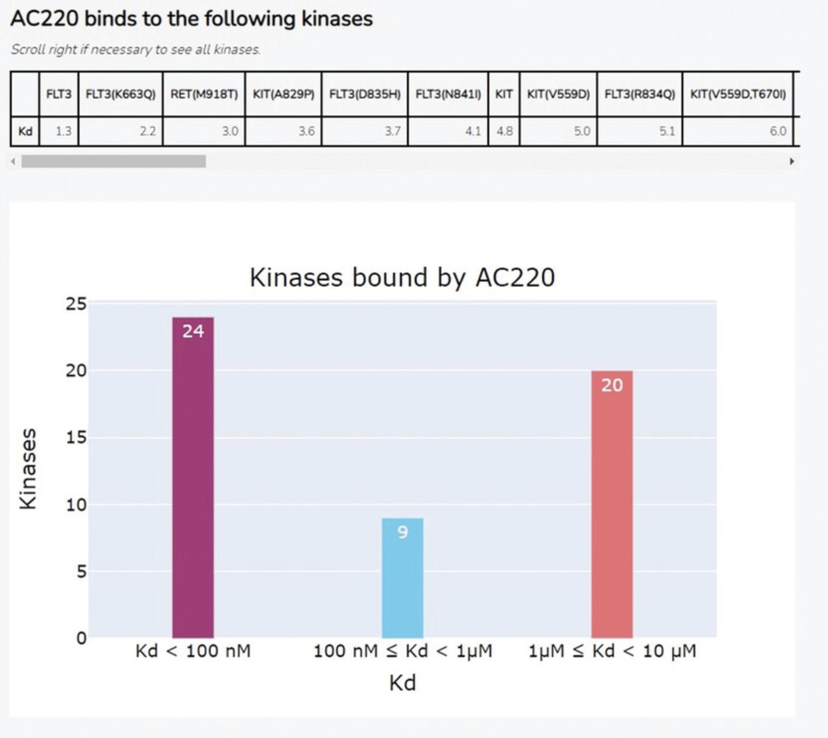
13.The Appyter will automatically begin execution. When execution has completed, as indicated by the “Success” box at the top of the page, scroll down to the section titled “Generate table and barchart of kinases for small molecule input from KINOMEscan data, with either equilibrium dissociation constant Kd or % Control” to view the results (Fig. 46). The table shows the top-ranked kinases bound by the input small molecule, based on either % control or Kd values; the bar chart shows the distribution of % control or Kd values among all kinases bound by the input small molecule.
Querying a kinase list
14.Navigate to the KINOMEscan Data Visualization Appyter at https://appyters.maayanlab.cloud/#/KINOMEscan and click the “Start Appyter” button to view the input form (see Fig. 44).
15.Scroll to the section titled “Upload or Enter a List of Kinases”. You may either upload a text file (.txt) using the “Upload kinase list” box or type a list of kinases into the “Input kinase list” box. Each row of either the file upload or text input should have only one kinase. Scroll to the bottom of the input form and click the blue “Submit” button.
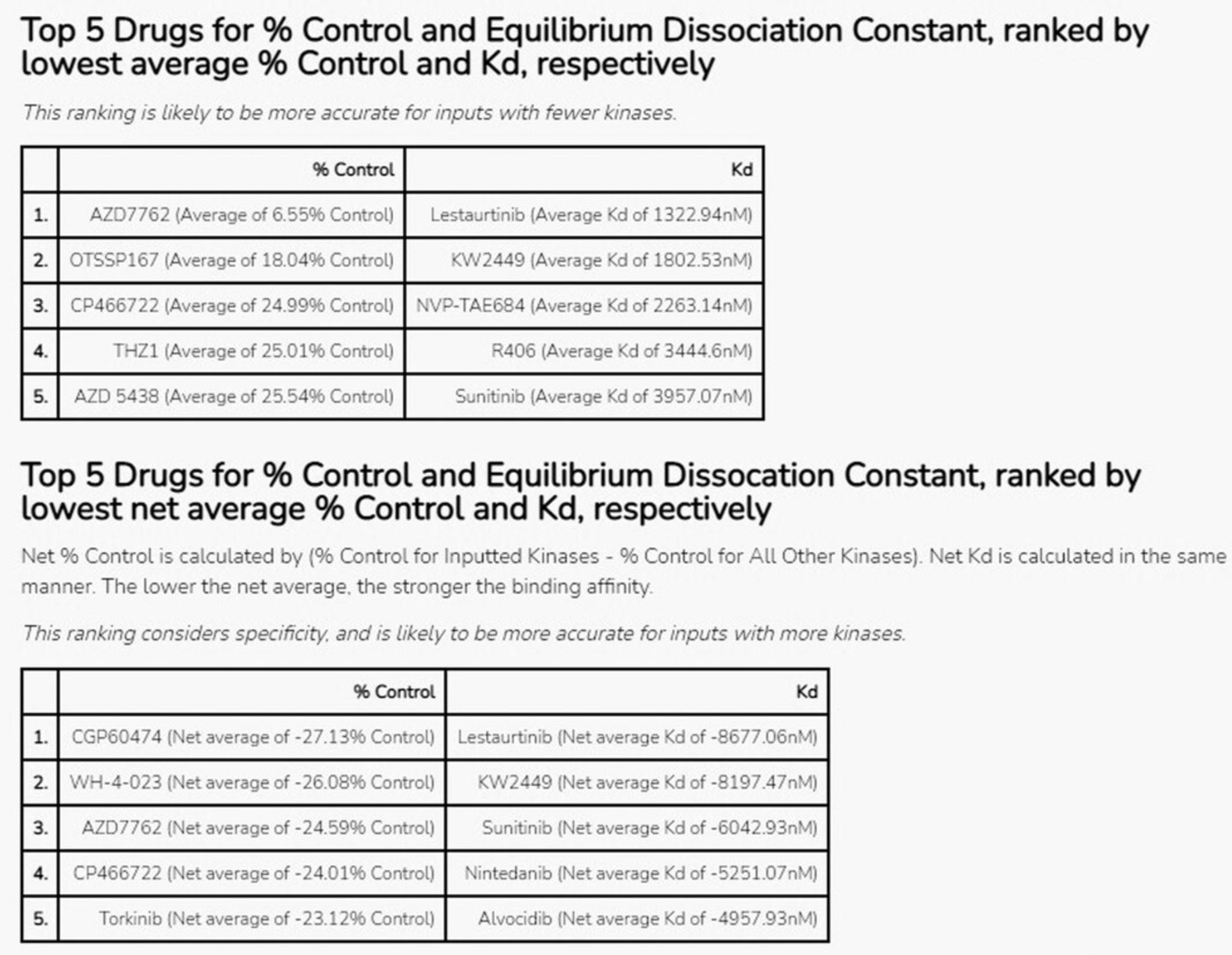
16.The Appyter will automatically begin execution. When execution has completed, as indicated by the “Success” box at the top of the page, scroll down to the section titled “Generate ranked lists of drugs for inputted or uploaded kinases” to view the results (Fig. 47), which show the top 5 drugs that bind to the kinases in the input list by average % control and Kd, as well as by net average % control and Kd. Net values are calculated by subtracting the average % control or Kd value across all kinases from the average % control or Kd for only the input kinases.
Querying a gene list
17.Navigate to the KINOMEscan Data Visualization Appyter at https://appyters.maayanlab.cloud/#/KINOMEscan and click the “Start Appyter” button to view the input form (see Fig. 44).
18.Scroll to the section titled “Upload or Enter a Gene/Protein List”. You may either upload a text file (.txt) using the “Upload gene/protein list” box, or type in a list of genes to be queried into the “Input gene/protein list” box. Each row of either the file upload or text input should have only one kinase.
19.In the “Number of top kinases to consider” input box, enter in how many top kinases you would like to see in the results. The default value is 10.Then, scroll to the bottom of the input form and click the blue “Submit” button.
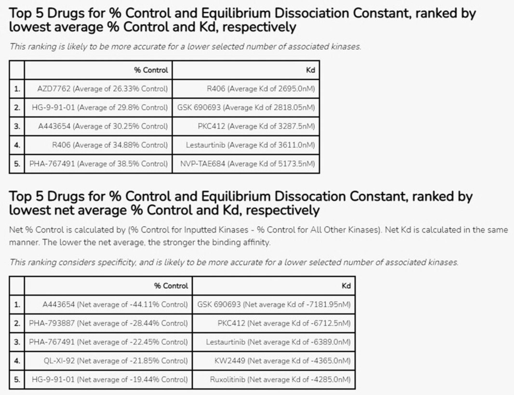
20.The Appyter will automatically begin execution. When execution has completed, as indicated by the “Success” box at the top of the page, scroll down to the section titled “Perform Kinase Enrichment Analysis on the inputted or uploaded genes” (Fig. 48). The tables show the results of performing kinase enrichment analysis on the input gene list. The top five drugs that bind to kinases coded by the input genes are displayed, based on average % control and Kd values, as well as based on net average % control and Kd. Net values are calculated by subtracting the average % control or Kd value across all kinases from the average % control or Kd for only the input kinases.
Basic Protocol 6: LINCS PROTEOMICS: THE P100 AND GCP ASSAYS
The LINCS Proteomic Characterization Center for Signaling and Epigenetics (PCCSE) examined the effects of small molecule and genetic perturbations on the proteome and epigenome (Litichevskiy et al., 2018). Changes in phospho-signaling and chromatin states were measured using two liquid chromatography mass spectrometry (LCMS) assays. The P100 assay measures the levels of 96 widely studied cell signaling peptides and phosphopeptides, which serve as a reduced representation of the signalome. The global chromatin profiling (GCP) assay measures post-translational histone modifications in bulk chromatin, which enables the generation of epigenetic signatures corresponding to various perturbations. These LINCS proteomics datasets are hosted on the PanoramaWeb (Sharma et al., 2018) and CLUE.io platforms (Subramanian et al., 2017). The datasets produced by the PCCSE can be visualized in the form of heatmaps produced with the Morpheus matrix visualization and analysis software (https://software.broadinstitute.org/morpheus/).
Necessary Resources
Hardware
Desktop or a laptop computer, or a mobile device, with a fast Internet connection
Software
- An up-to-date web browser such as Google Chrome (https://www.google.com/chrome/), Mozilla Firefox (https://www.mozilla.org/en-US/firefox/), Apple Safari (https://www.apple.com/safari/), or Microsoft Edge (https://www.microsoft.com/en-us/edge)
1.Navigate to the LINCS Panorama Repository dashboard at https://panoramaweb.org/project/LINCS/begin.view. The homepage provides an overview of the LINCS PCCSE assays and data. (Fig. 49)
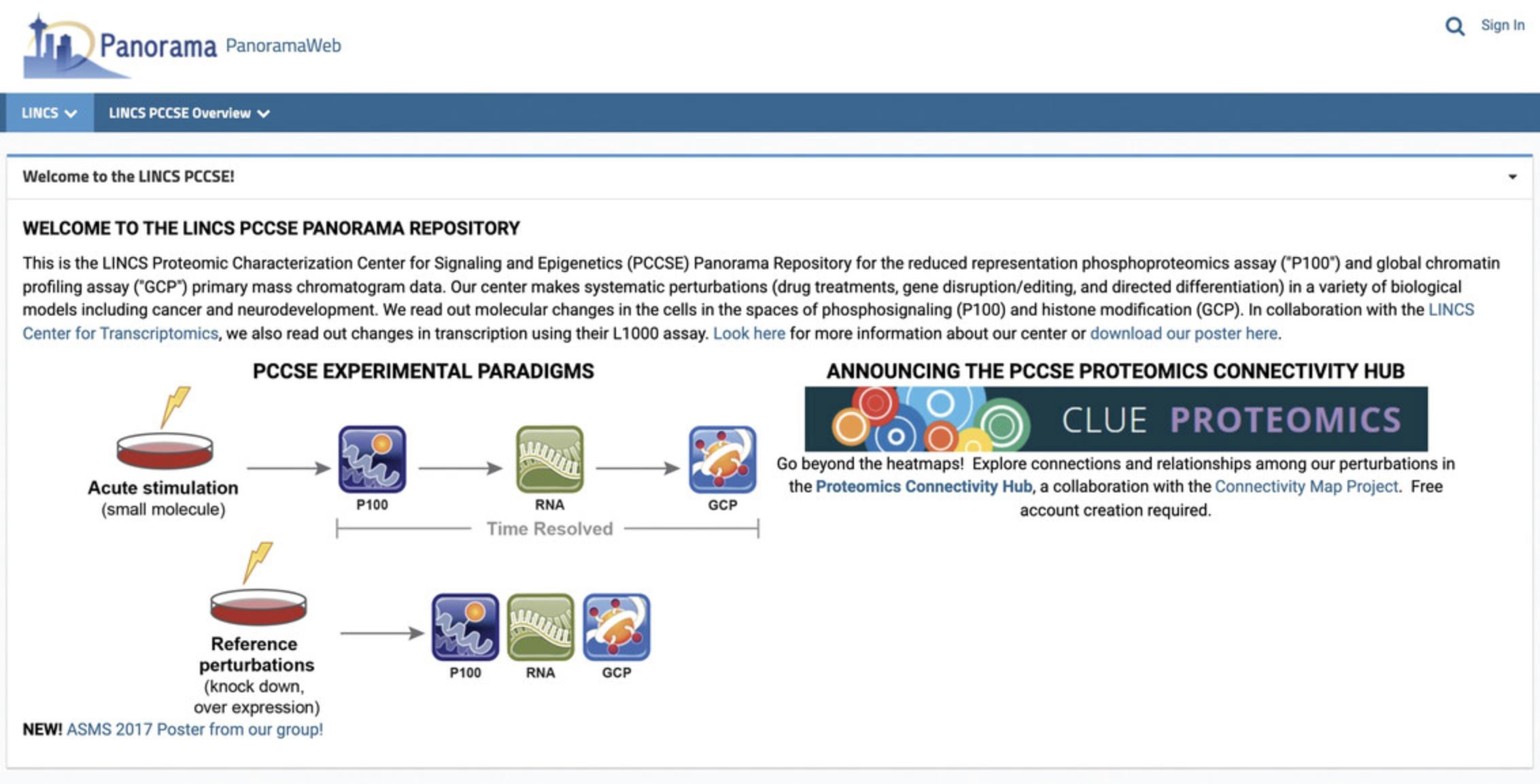
2.Hover over the “LINCS PCCSE Overview” drop-down menu at the top of the page and click on any of the selections to view standard operating procedures (SOPs), quality control, internal standards, and any posters or presentations created for introducing the PCCSE data.
Accessing P100 and GCP data with Panorama
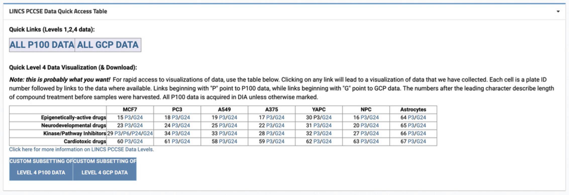
3.Scroll to the “LINCS PCCSE Data Quick Access Table” section. Under the “Quick Links” heading, click on the “ALL P100 DATA” and “ALL GCP DATA” buttons (Fig. 50). The new page will display data tables containing all metadata and download links for the P100 or GCP datasets, respectively.
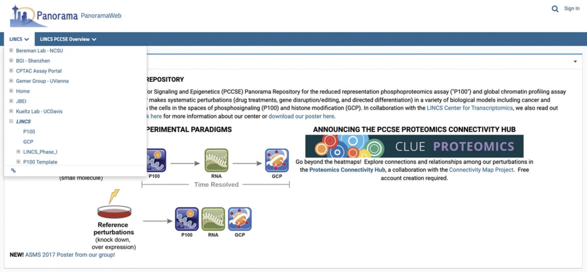
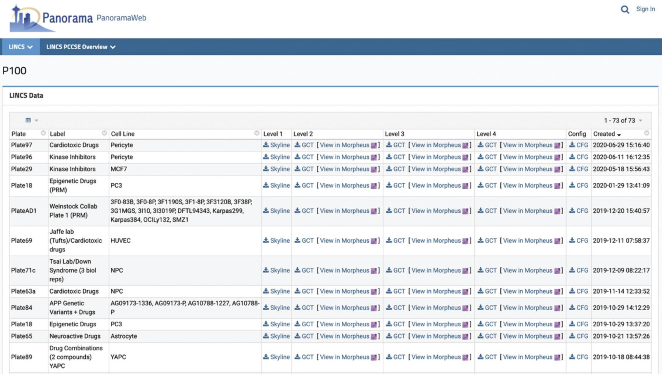
4.On the assay-specific data page, under the “LINCS Data” section, each dataset is available in four different levels (Figs. 52 and 53).
- a.Click on the Skyline link for the Level 1 data for any dataset to view a data table of all precursors in the dataset in a new page (Fig. 54).
- b.Click on the download icon for the Level 2-4 data for any dataset to directly download the GCT files.
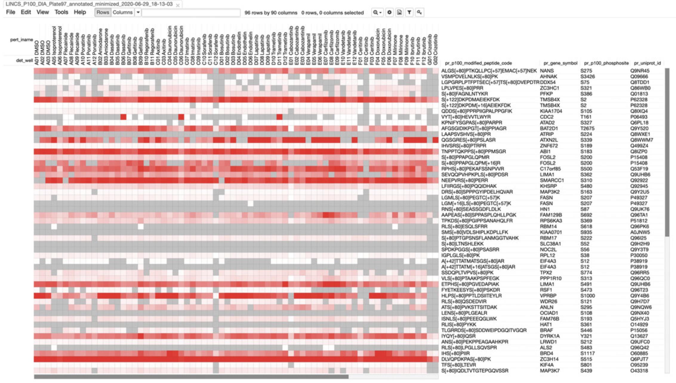
- c.Click on the “View in Morpheus” link for the Level 2-4 data for any dataset to see a heatmap of the corresponding assay data (Fig. 55). The columns correspond to various drug treatments, while the rows correspond to genes. Refer to steps 9-12 below to understand the heatmaps.

5.Scroll to the “LINCS PCCSE Data Quick Access Table” section to view other datasets. Click on any link to be taken to the dataset page.
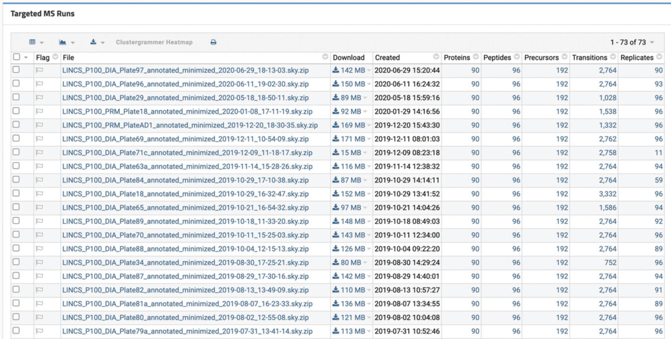
6.Scroll to the “Targeted MS Runs” section for a list of annotated mass spectrometry data for each plate (Fig. 56). Click on any file name to download the file. To view a list of all proteins, peptides, precursors, transitions, and replicates in the dataset, click on the number corresponding to each column. Use the grid at the top of the table to customize the table, create a chart, or export the data table.
7.Scroll to the “Mass Spec Search” section to search for specific proteins, peptides, or modifications in the data using the search box (Fig. 57).

8.Scroll to the “Messages” section to view updates or corrections to the datasets (Fig. 58).
Visualizing LINCS Proteomics data with Morpheus
9.Under the “Quick Level 4 Data Visualization” heading, click on any link in the table to view visualizations of P100 and/or GCP data for the indicated drug class and cell line in Morpheus, similar to the results from step 4c above (see Fig. 55). The name of the dataset displayed is shown on the tab heading at the top of the page.
10.Hover over any box to see the value corresponding to the effect of the specified drug on the histone or peptide. The names of the drug, well number, and histone/peptide will also appear at the top of the heatmap.
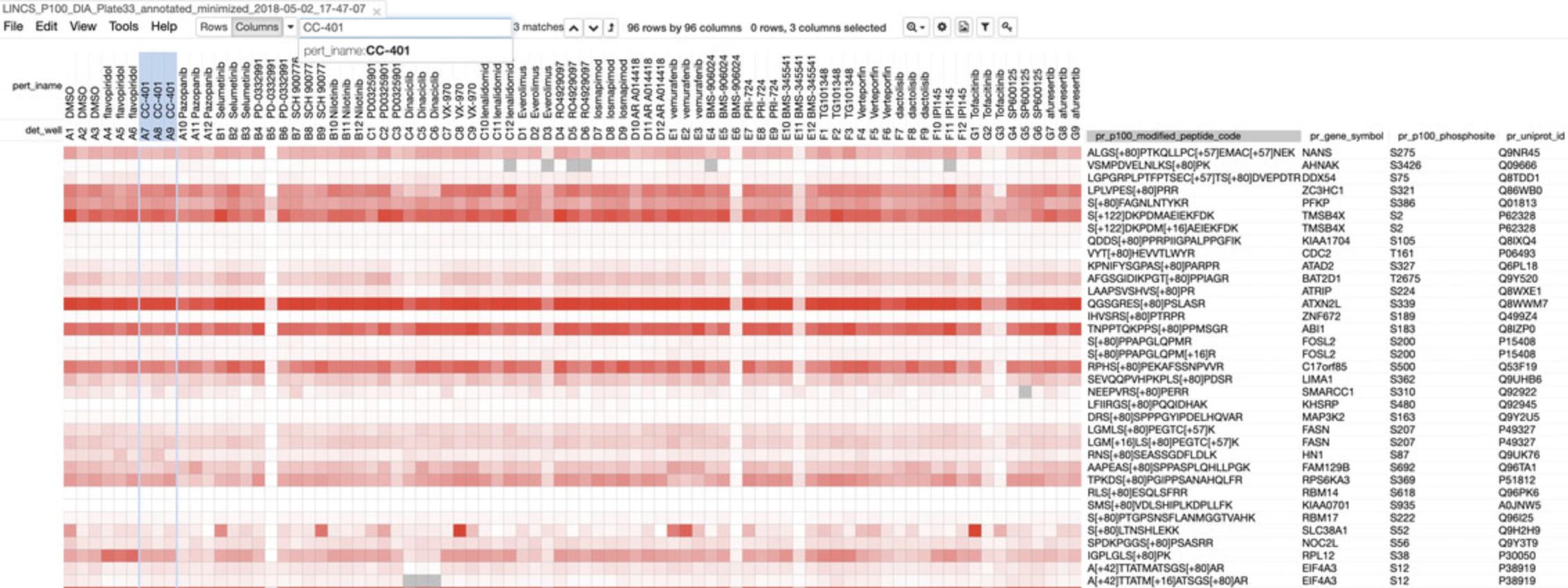
11.Use the search bar at the top of the page to filter out specific data entries. Select whether to filter by rows or columns, and which category to filter by, then enter in the query term. If the term appears in the data, the term and the column or row category it belongs to will automatically appear in the search bar. Use the up and down arrow keys next to the search bar to move between search results. Click the “Matches at Top” button to automatically move selected entries towards the top left of the heatmap (Fig. 59).

12.Use the additional tool options at the top of the heatmap to customize or save the image.
- a.Use the zoom drop-down menu to zoom into, or out of the heatmap.
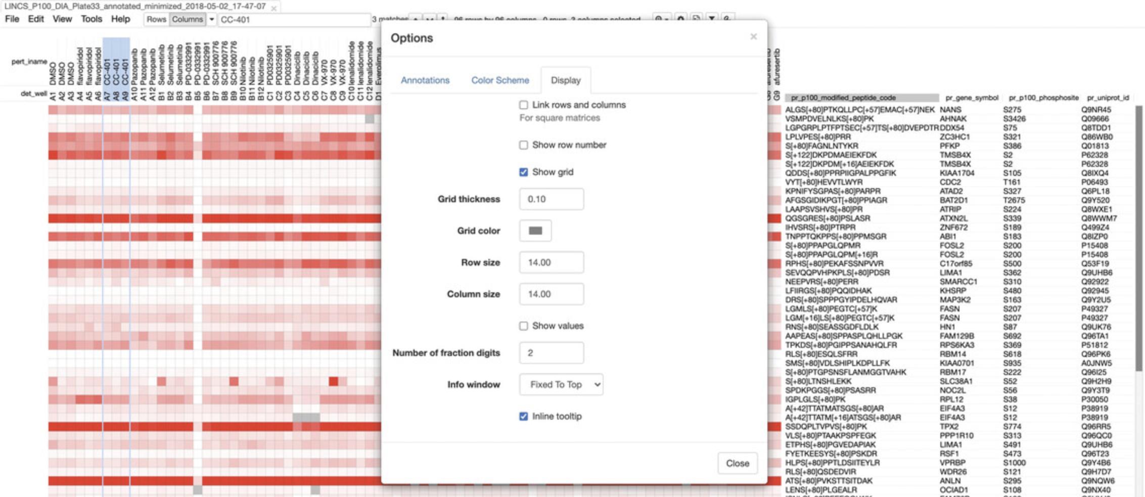
- b.Click the options button to customize the annotations, color scheme, or display settings for the heatmap (Fig. 60).
- c.Click the save button to save the heatmap to PNG, PDF, or SVG file format.
- d.Click the color key button to view the range of data values, and the color to which each value corresponds on the heatmap.
Basic Protocol 7: THE LINCS JOINT PROJECTS (LJPs)
The two LINCS Joint Projects involve collaborations between several LINCS DSGCs and the DCIC. The Broad-HMS LINCS Joint Project explores the dose-dependent sensitivities of six nonmalignant and cancerous breast tissue cell lines to 107 small molecule perturbagens applied at six different doses. The MEP-HMS LINCS Joint Project assessed the dose-dependent responses of 72 nonmalignant and cancerous breast tissue cell lines to 139 small molecule and antibody perturbagens applied at nine different doses. Data from both joint projects are available from the GR Browser (Clark et al., 2017) and the LINCS Joint Project Breast Cancer Network Browser (Niepel et al., 2017). The aim of both projects was to explore the dose-dependent responses of human cells to a focused set of common perturbations under common conditions with multiple readouts. This basic protocol provides a tutorial about how to access and analyze the data generated by these joint projects, as well as the associated software tools developed to analyze these datasets.
Necessary Resources
Hardware
Desktop or a laptop computer, or a mobile device, with a fast Internet connection
Software
- An up-to-date web browser such as Google Chrome (https://www.google.com/chrome/), Mozilla Firefox (https://www.mozilla.org/en-US/firefox/), Apple Safari (https://www.apple.com/safari/), or Microsoft Edge (https://www.microsoft.com/en-us/edge)
Viewing the dose-response grid with the GR Browser
1.Navigate to the GR Browser website at http://www.grcalculator.org/grbrowser/. By default, the page will display the dose-response grid of the Broad-HMS LINCS Joint Project dataset (Fig. 61).
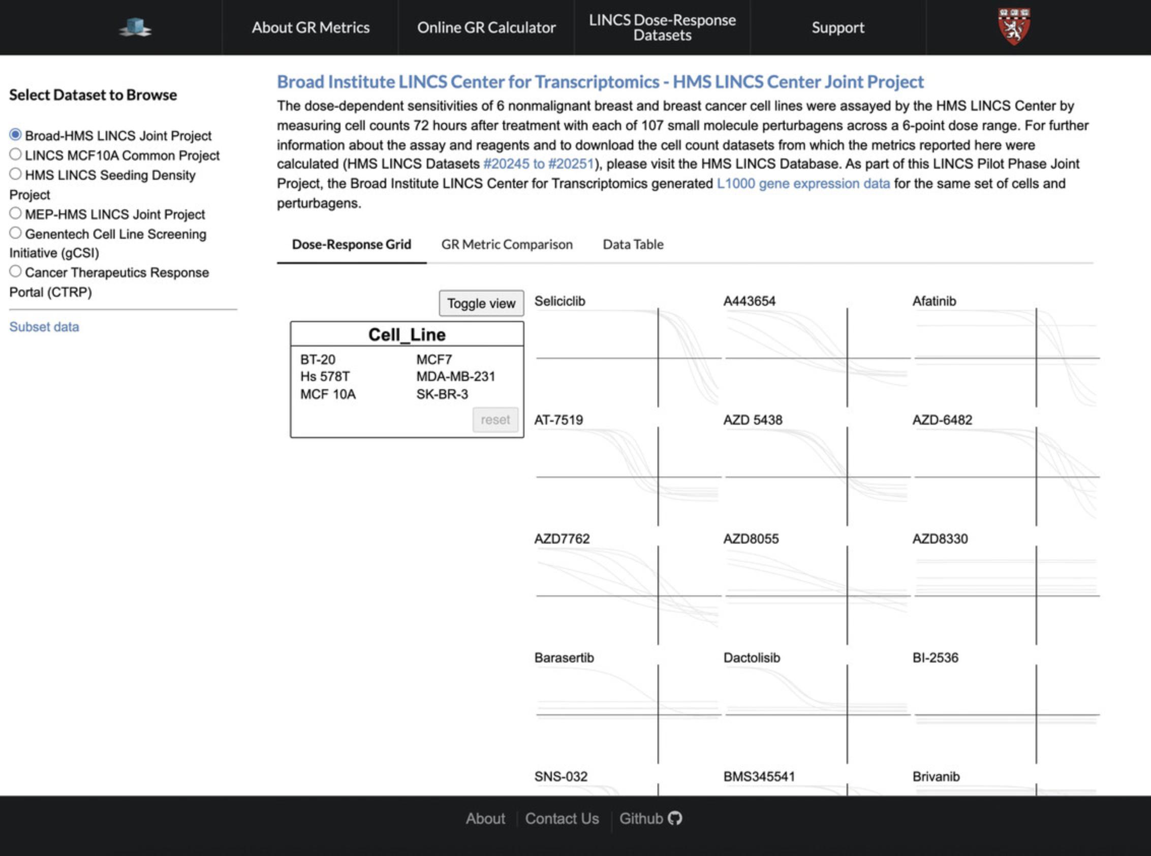
2.The Dose-Response Grid tab shows the dose-response curves corresponding to each cell line compiled for each compound.
3.Choose a dataset to explore using the “Select Dataset to Browse” menu on the left of the screen; the two LINCS Joint Projects are the “Broad-HMS LINCS Joint Project” and the “MEP-HMS LINCS Joint Project”. To view only data corresponding to a specific molecule or cell line, click the “Subset Data” button underneath the dataset list, and enter in the relevant molecule or cell line.
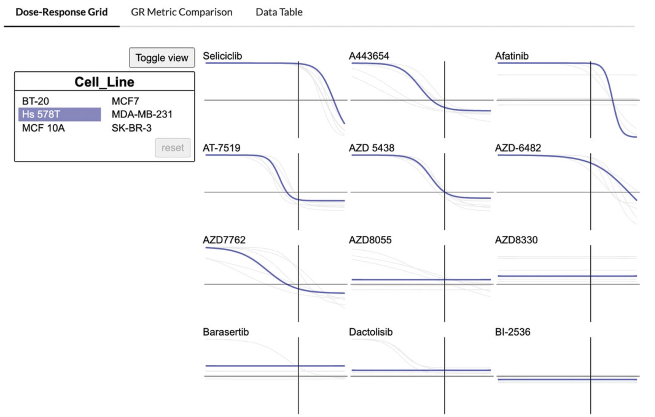
4.Hover over a cell line in the floating box titled “Cell_Line” to highlight the cell line-specific dose-response curves (Fig. 62).
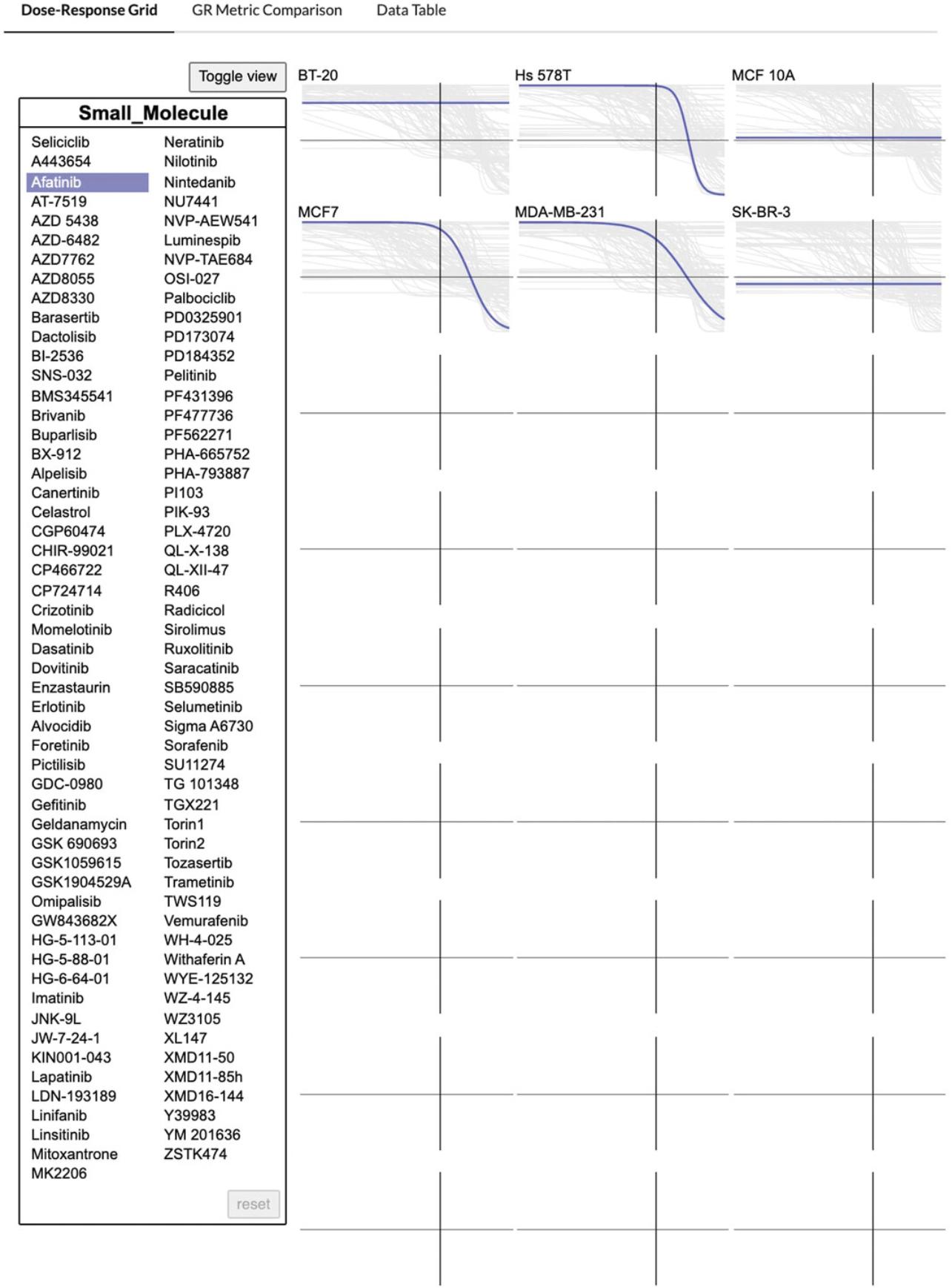
5.Click “Toggle View” to switch to viewing the dose-response curves for each compound compiled by cell line. Hover over any compound name in the floating box to highlight the compound-specific dose curves in the grid (Fig. 63).
Comparing GR metrics with the GR Browser
6.The GR Metric Comparison tab provides comparative visualizations of different dose-response metrics across different cell lines and small molecules (Fig. 64). By default, a boxplot is displayed, showing the GR50 measurements for the first nine small molecules by alphabetical order.
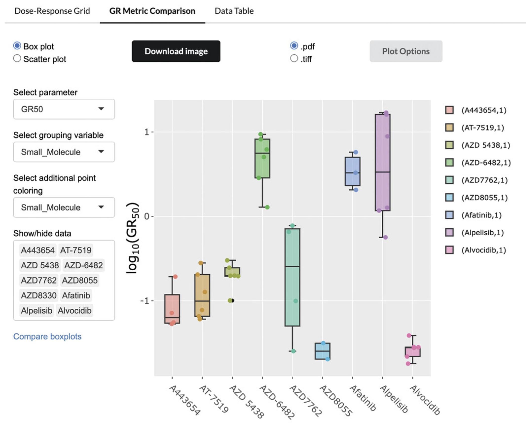
7.Use the menu on the left side of the tab to select either a boxplot or a scatterplot visualization, then choose a metric to visualize using the “Select parameter” drop-down menu. The following GR metrics are available:
-
GR50: Concentration at which the effect reaches a GR value of 0.5 based on interpolation of the fitted curve.
-
GRmax: Effect at the highest tested concentration.
-
GRinf: GR(c → ∞): Effect at infinite concentration based on extrapolation of the fitted curve, which reflects asymptotic drug efficacy. Note that GRinf can differ from GRmax if the measured dose-response does not reach its plateau value.
-
GEC50: Drug concentration at half-maximal effect, which reflects the potency of the drug.
-
hGR: Hill coefficient of the sigmoidal curve, which reflects how steep the dose-response curve is.
-
GRAOC: Area over the dose-response curve, which is the integral of 1–GR(c) over the range of concentrations tested.
8.Choose to compare either small molecules or cell lines using the “Select grouping variable” drop-down menu, then enter in the specific molecules or cell lines you would like to compare in the “Show/hide data” box. By default, the first ten options in alphabetical order are displayed.
9.Click on the “Plot Options” button to display options for customizing the plot size, labels, and margins.
10.Click the “Download Image” button above the plot to download the plot as either a TIFF (.tiff) or PNG (.png) file.
Viewing dose-response data and metadata in the GR Browser
11.The Data Table tab displays the full table of dose-response metrics and metadata for each perturbation (Fig. 65).
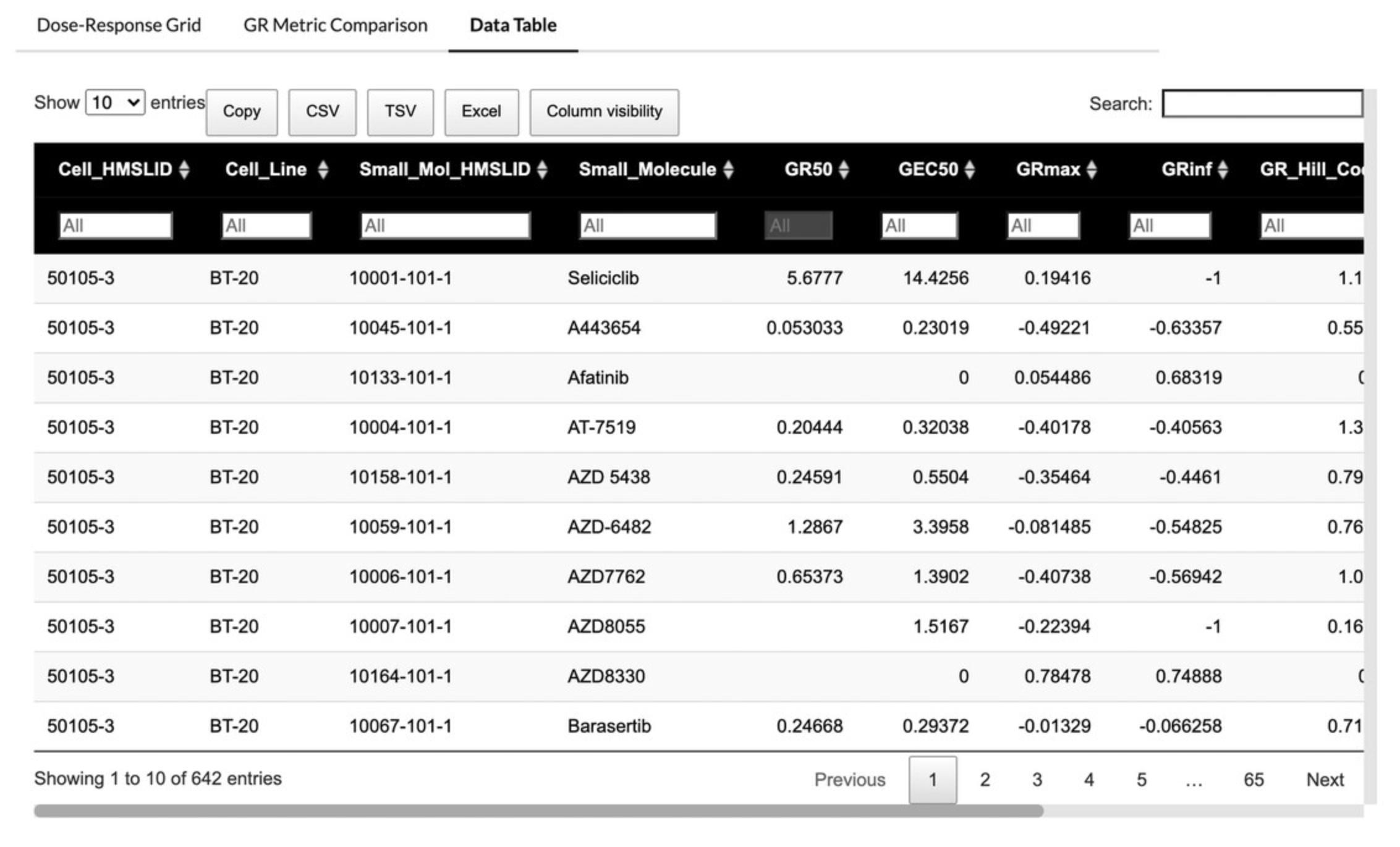
12.Click the arrows next to any column name in the table to sort the table by the values in that column in ascending or descending order.
13.Enter a specific value into the box below each column name to filter the values in that column, or enter a value into the search box at the top right of the tab to search across all columns. In the example figure (Fig. 66), the data is filtered by AZD compounds using the search box at the top right, and by the BT-20 cell line using the “Cell_Line” column.
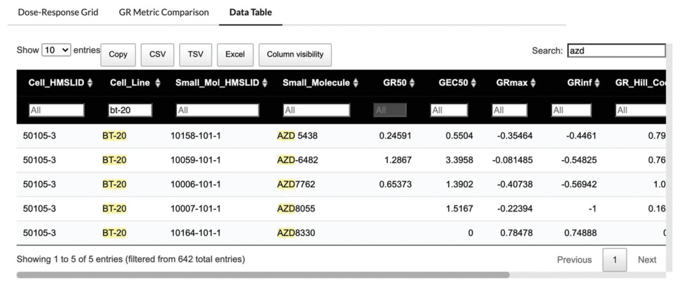
14.Copy the table or download the table as a CSV (.csv), TSV (.tsv), or Excel (.xlsx) file using the corresponding buttons above the table.
Accessing the LINCS Joint Project data with the HMS LINCS database
15.Navigate to the HMS LINCS database at https://lincs.hms.harvard.edu/db/datasets/. This page displays a table containing all available datasets from the HMS LINCS DSGC, including the dataset ID, dataset name, and the type of data available.
16.In the search box near the top of the page, enter in “LINCS Joint Project”. The table will then filter only the 17 Broad-HMS LINCS Joint Project datasets (Fig. 67).
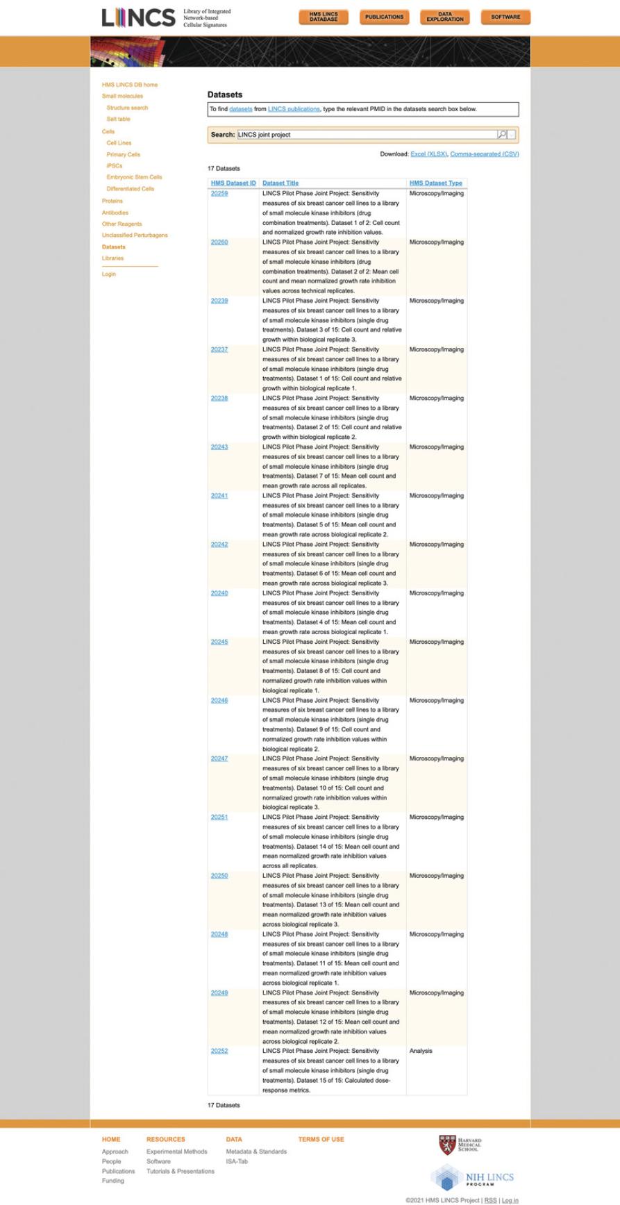
17.Click on any ID in the “HMS Dataset ID” column to view a specific LJP dataset. The data and metadata are divided into various detailed tabs, each of which can be downloaded as Excel (.xlsx) or CSV files by using the download links in the top right corner of the tab. By default, the “Detail” tab is shown on the new page, which provides project information and metadata (Fig. 68).
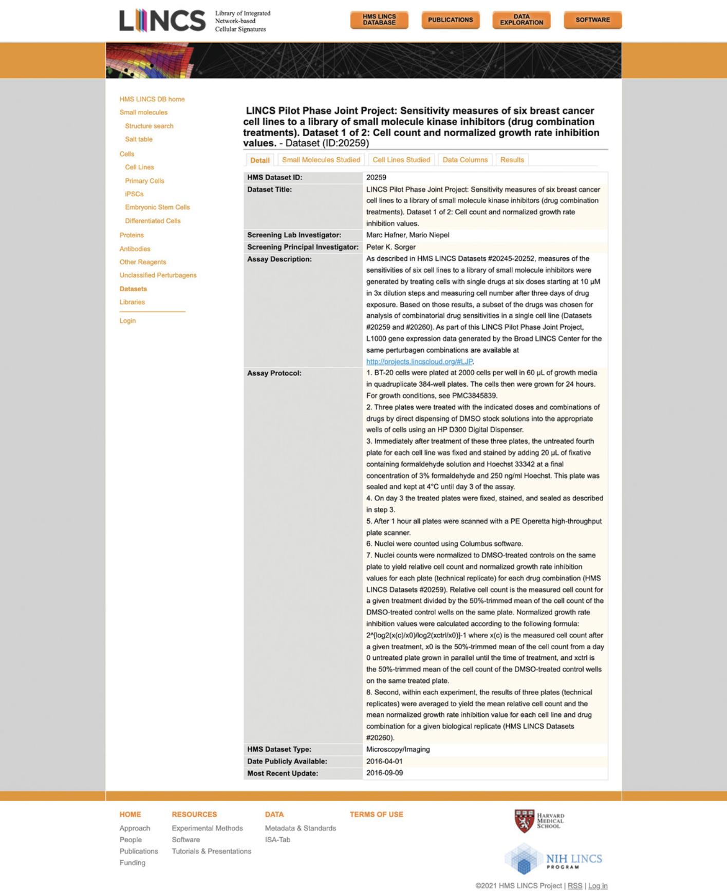
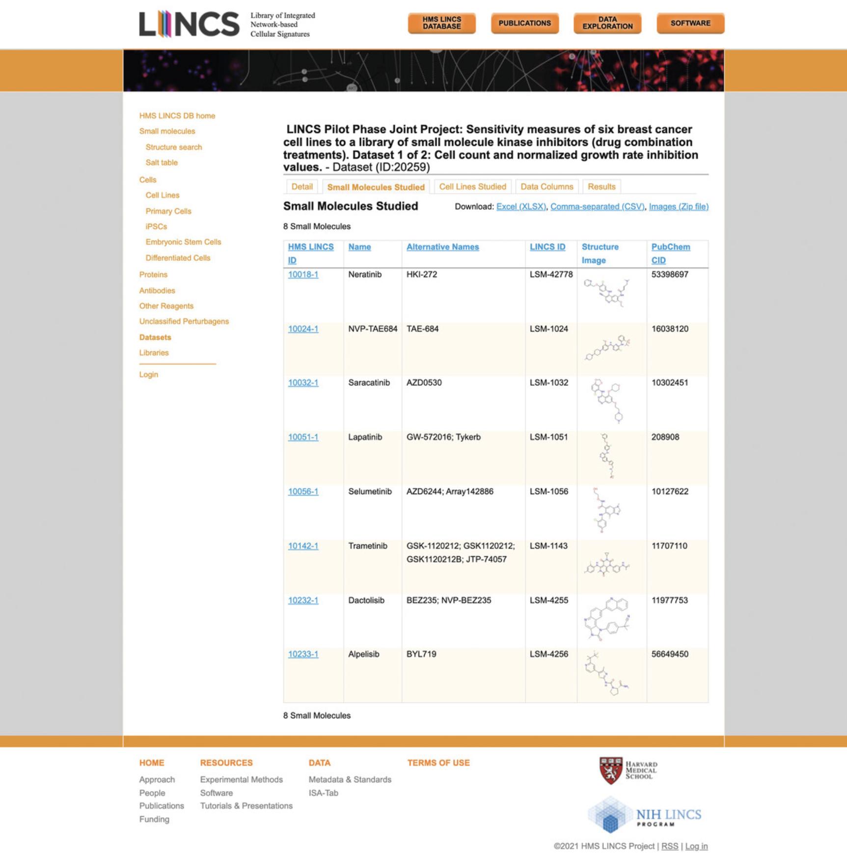
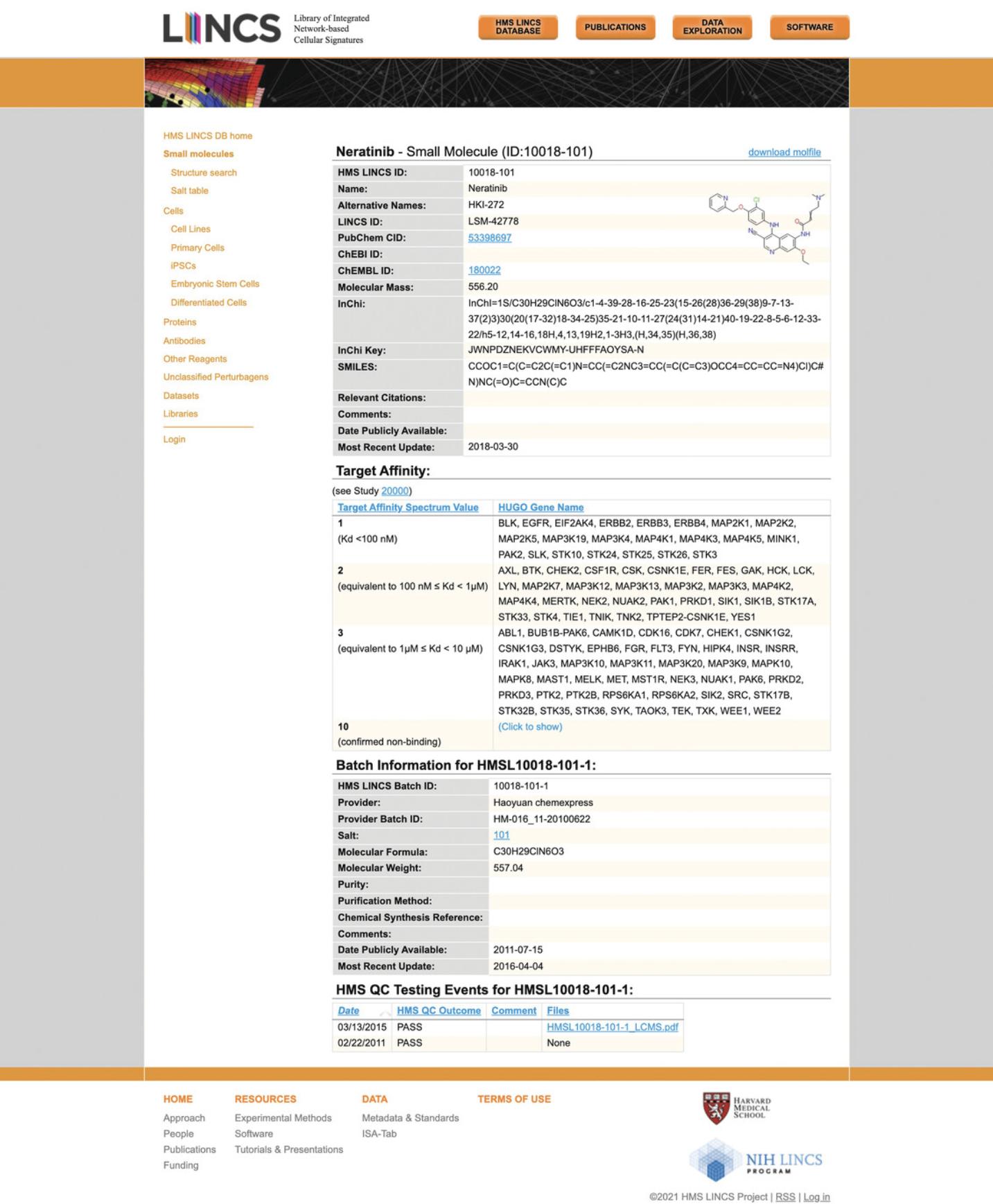
18.Click the “Small Molecules Studied” tab to view the various small molecules profiled by the LJP in the chosen dataset (Fig. 69). Click on any of the small molecule IDs under the “HMS LINCS ID” column to display all available metadata on the molecule; the example figure shows metadata for neratinib (Fig. 70).
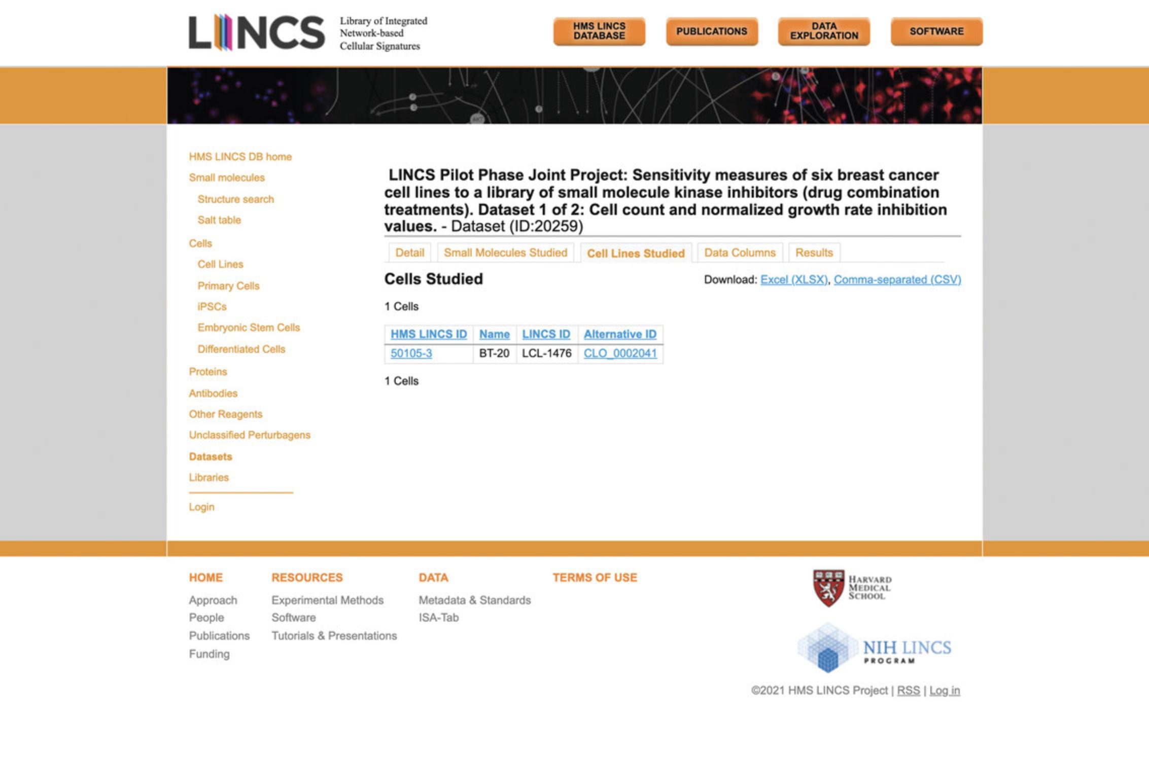
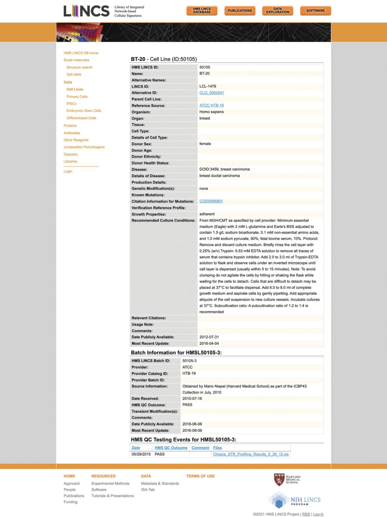
19.Click the “Cell Lines Studied” tab to view the cell lines corresponding to the chosen dataset (Fig. 71). Click on an ID under the “HMS LINCS ID” column to display metadata on the chosen cell line; the example figure shows the cell line BT-20 (Fig. 72).
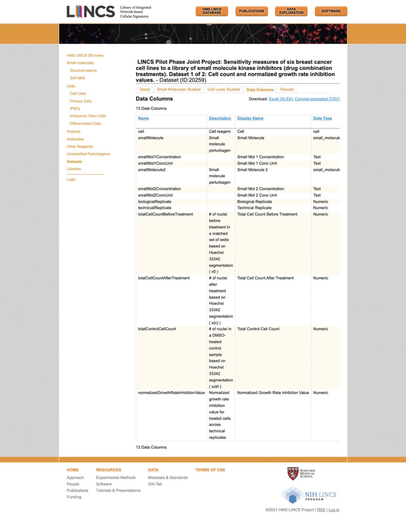
20.Click the “Data Columns” tab to view the descriptions of each column in the results table for the given dataset (Fig. 73).
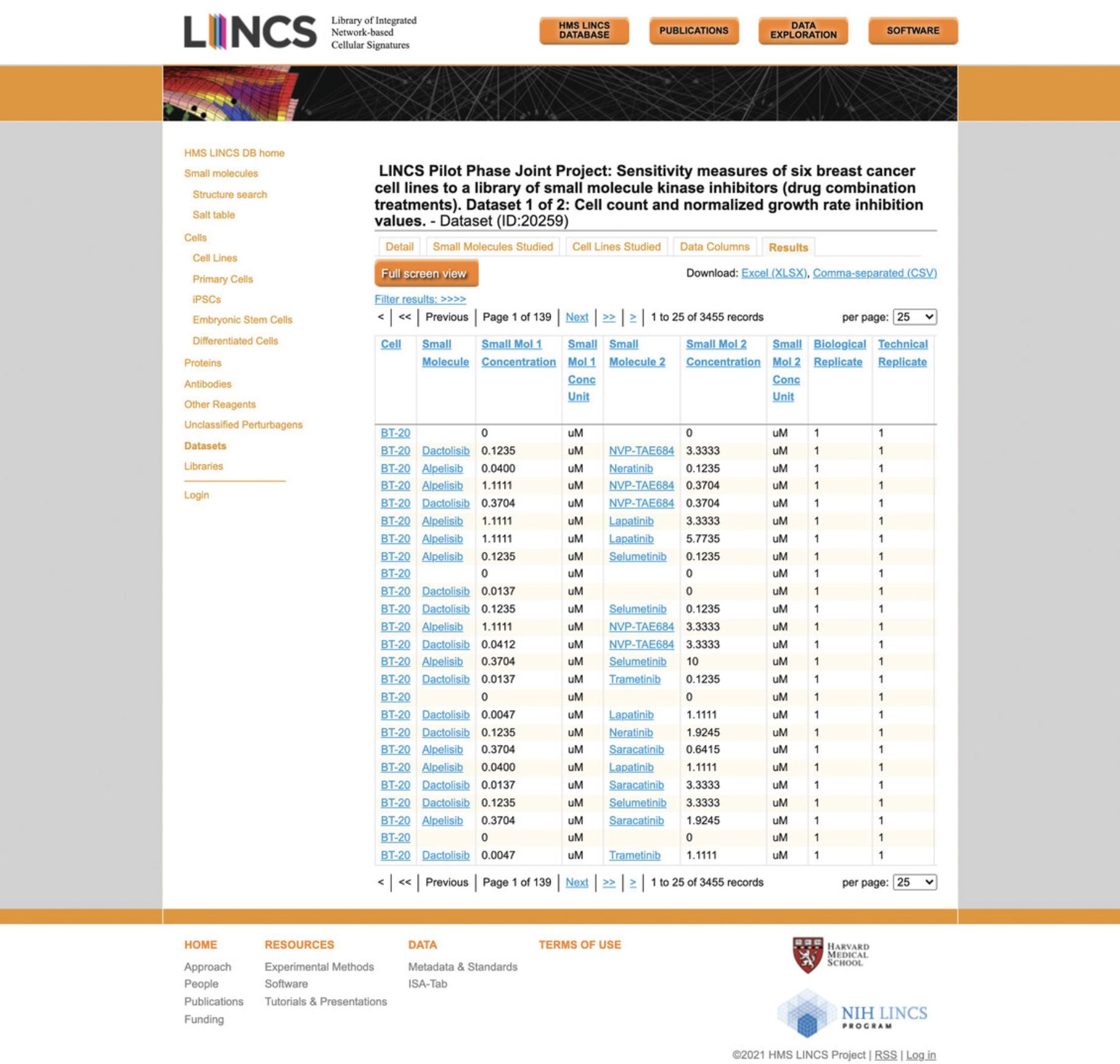
21.Click the “Results” tab to view the actual data contained in the dataset (Fig. 74). Each row represents an experimental replicate for a single or combination small molecule perturbation that was applied to the specified cell line.
Accessing the LINCS Joint Project Breast Cancer Network Browser
22.Navigate to the LINCS Joint Project Breast Cancer Network Browser (BCNB) at https://maayanlab.cloud/LJP/. The homepage displays a network visualizing all perturbational gene expression signatures obtained from the LJP (Fig. 75).
-
By default, the shape of each point represents the cell line, the size represents the approximate GR value of the small molecule, and the color represents the drug class of the small molecule. The legend on the left side of the network provides all relevant mappings.
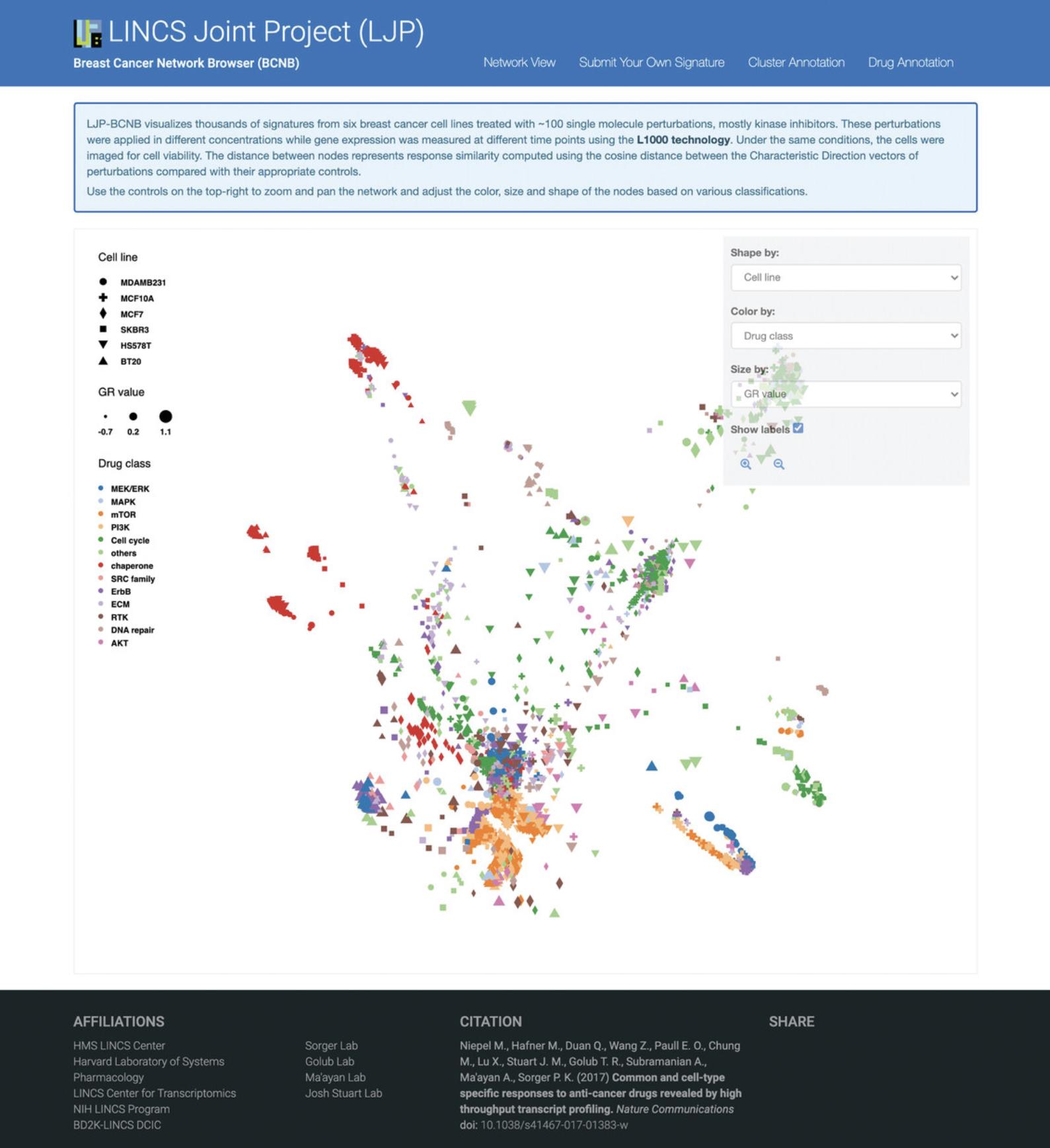
23.Use the drop-down menu on the right side to adjust the shape, color, and size.
-
The shape may be determined by cell line, timepoint, or concentration.
-
The color may be determined by several perturbational metrics and metadata, including GR value,p-value, cell line, timepoint, or concentration. The color may also be determined by cellular function or role, or the most enriched term for the signature from several gene set libraries.
-
The size may be determined by GR value,p-value, timepoint, or concentration.
24.Select the “Show labels” box beneath the drop-down menu to see information on the corresponding signature when hovering over a specific point on the network.
25.Use the zoom controls below the “Show labels” box, or the scroll function on your system to zoom in or out of the network. Click and drag the network to pan.
Basic Protocol 8: THE LINCS DATA PORTALS
The LINCS Data Portals were developed by the DCIC and can be used for viewing, downloading, and analyzing data generated by the LINCS DSGCs. There are three versions of the LINCS Data Portal; the LINCS Data Portal version 1 (Koleti et al., 2018) and version 2 (Stathias et al., 2019), which both correspond to earlier releases of LINCS data, and SigCom LINCS (Evangelista et al., 2022). The LINCS Data Portal 2.0 contains an upgraded user interface and enhanced metadata annotation compared to version 1.The latest LINCS Data Portal, SigCom LINCS, contains the most recent 2021 release of LINCS data, and contains many other features including enhanced metadata and signature search, single gene search, signatures from other sources, and term search, as well as global visualizations of the LINCS data.
Necessary Resources
Hardware
Desktop or a laptop computer, or a mobile device, with a fast Internet connection
Software
- An up-to-date web browser such as Google Chrome (https://www.google.com/chrome/), Mozilla Firefox (https://www.mozilla.org/en-US/firefox/), Apple Safari (https://www.apple.com/safari/), or Microsoft Edge (https://www.microsoft.com/en-us/edge)
Using LINCS Data Portal Version 1
1.Navigate to the LINCS Data Portal website (Fig. 76): http://lincsportal.ccs.miami.edu/dcic-portal/.
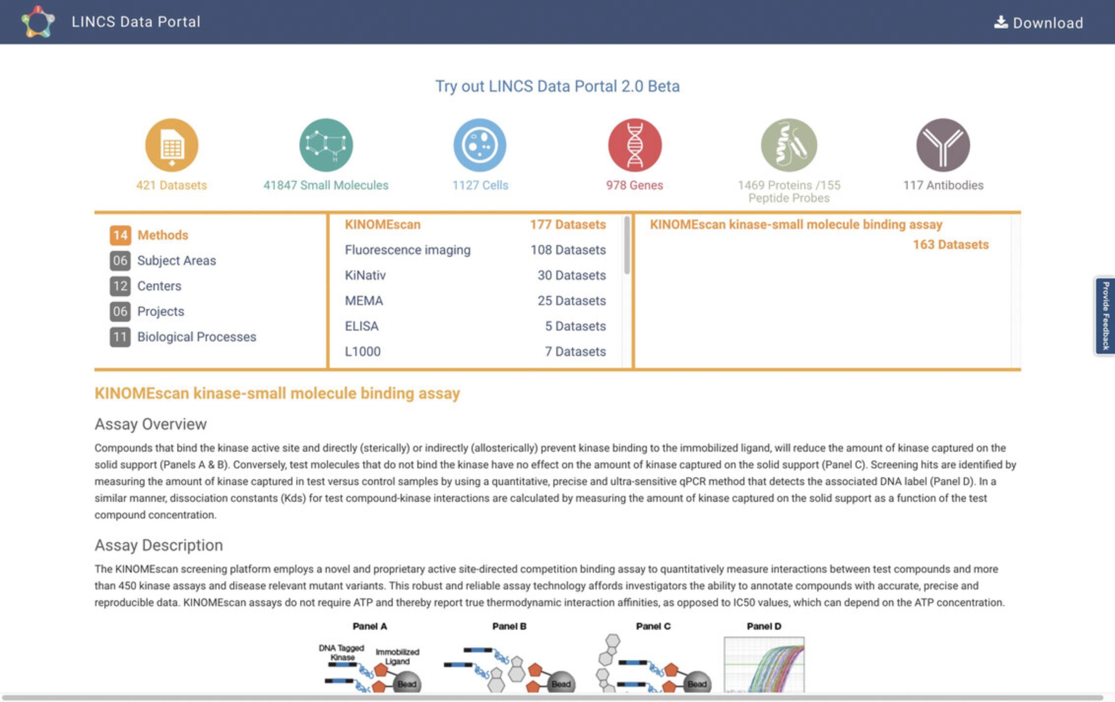
Selecting the L1000 data from the homepage
2.The left panel has Methods selected by default. In the center panel that lists the 15 available methods, click on “L1000”, and then in the right panel, click on “L1000 mRNA profiling assay” (Fig. 77). Statistics for the associated datasets, small molecules, cells, and genes are displayed above this table. Clicking on any of these icons will navigate you to the L1000 data grouped by that category.
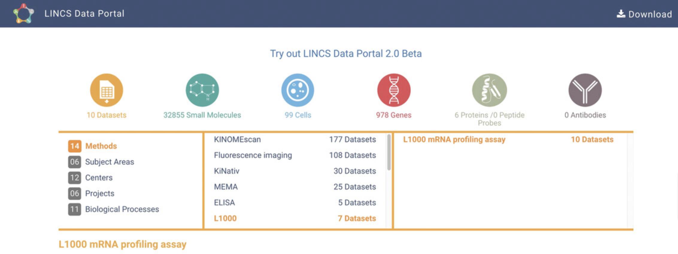
Viewing the L1000 datasets at a high level
3.Click on the “10 Datasets” option above the table on the homepage, to be navigated to an overview of the 10 available L1000 datasets (Fig. 78). By default, Table View of the results is provided, and this content can alternatively be displayed in List View. For each returned dataset, the associated LINCS Center, assay, method, subject area, and data level are provided.
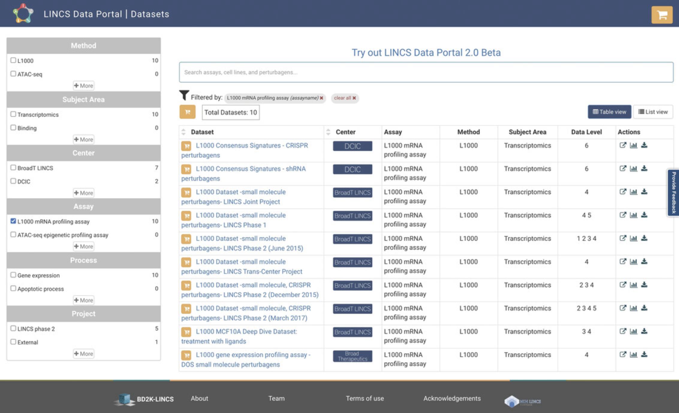
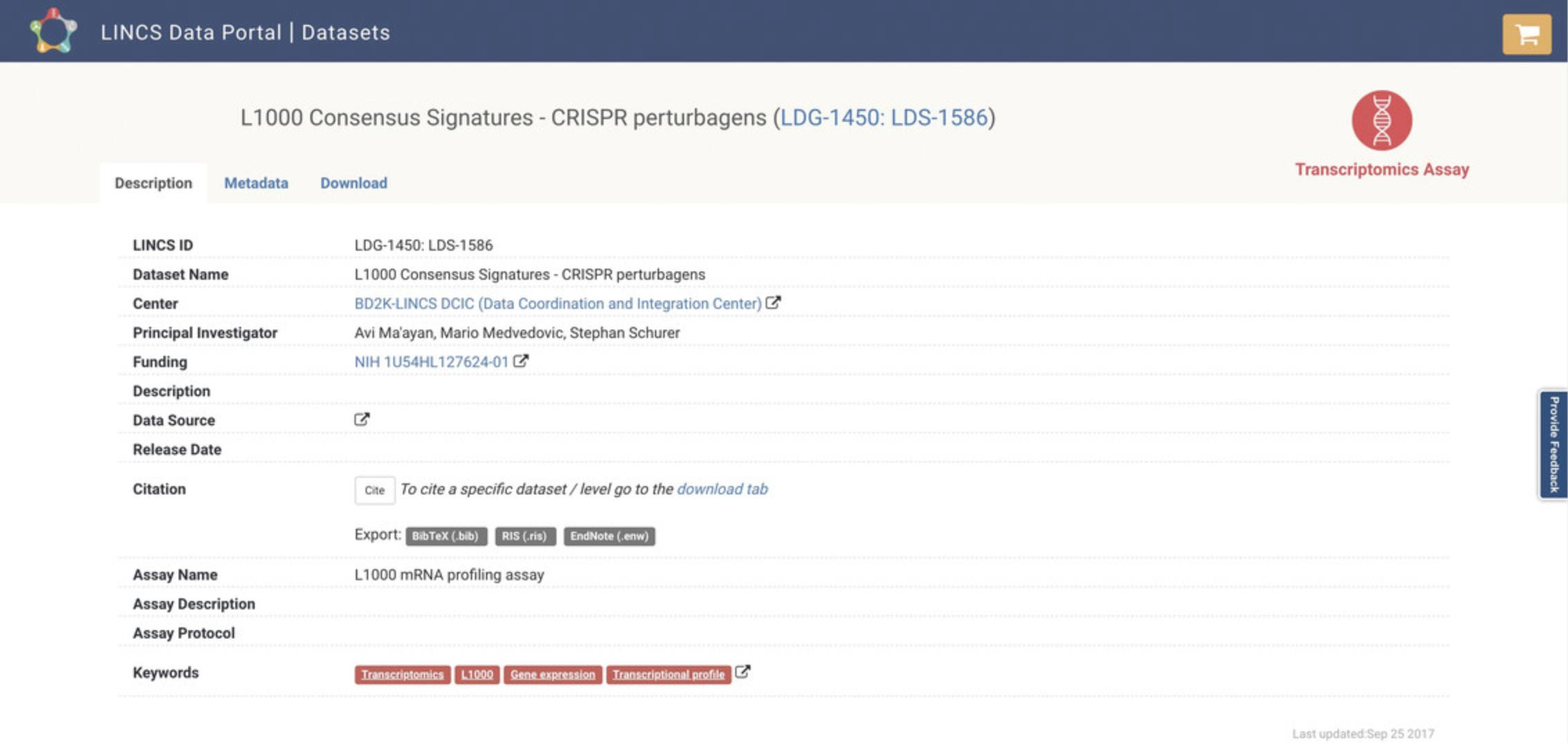
4.Use the search bar at the top of the page to query by keyword and use the menu on the left to filter datasets by Center, Project, and other criteria. Each result is associated with a hyperlink that can be clicked to display a detailed description and metadata, and a tab to download that dataset (Fig. 79). Additionally, action icons are listed for each entry, and these include Source Link, Dataset Statistics, and Download; each icon can be clicked to execute the selected action.
Viewing the L1000 datasets from a small-molecule perspective
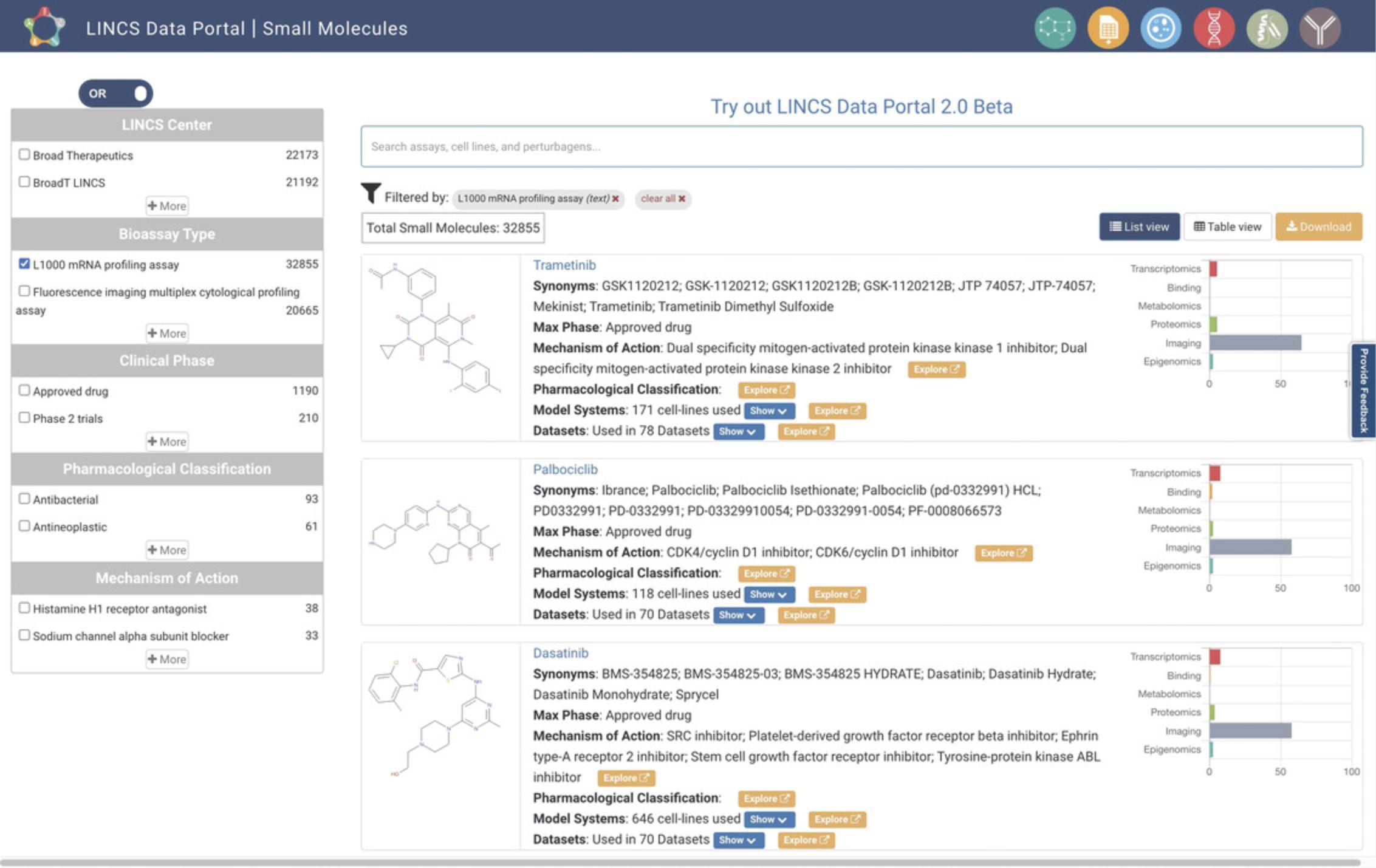
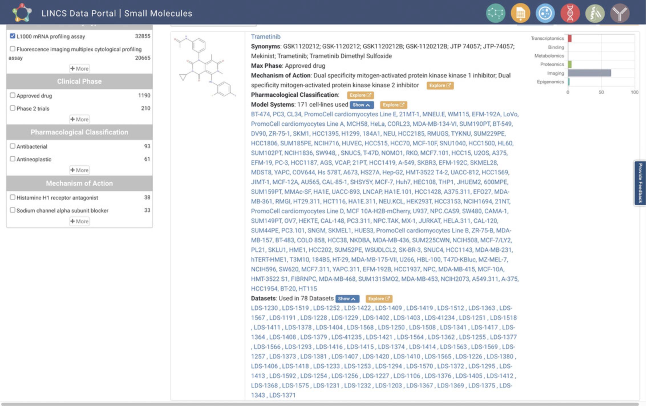
5.Starting from step 2, with the L1000 data having been selected on the homepage, click the Small Molecules icon on the homepage. This will navigate to a small-molecule-centric view of the L1000 data (Fig. 80). The results are displayed in Table View by default, and List View can alternatively be selected via the button above the results display. Each result lists the small molecule's name, its synonyms, most advanced phase of clinical approval (Max Phase), mechanism of action, pharmacological classification, model systems, and associated datasets. A bar plot for each result displays the experimental platforms of the datasets with which that small molecule is associated. Results can be searched by assays, cell lines, and other keywords via the search box above the results display. The results can also be filtered by LINCS Center, bioassay type, clinical phase, pharmacological classification, and mechanism of action using the menu on the left bar. Clicking on the blue “Show” buttons will expand the lists of model systems and datasets and provide a hyperlink to each (Fig. 81).
Viewing the L1000 datasets from a cell perspective
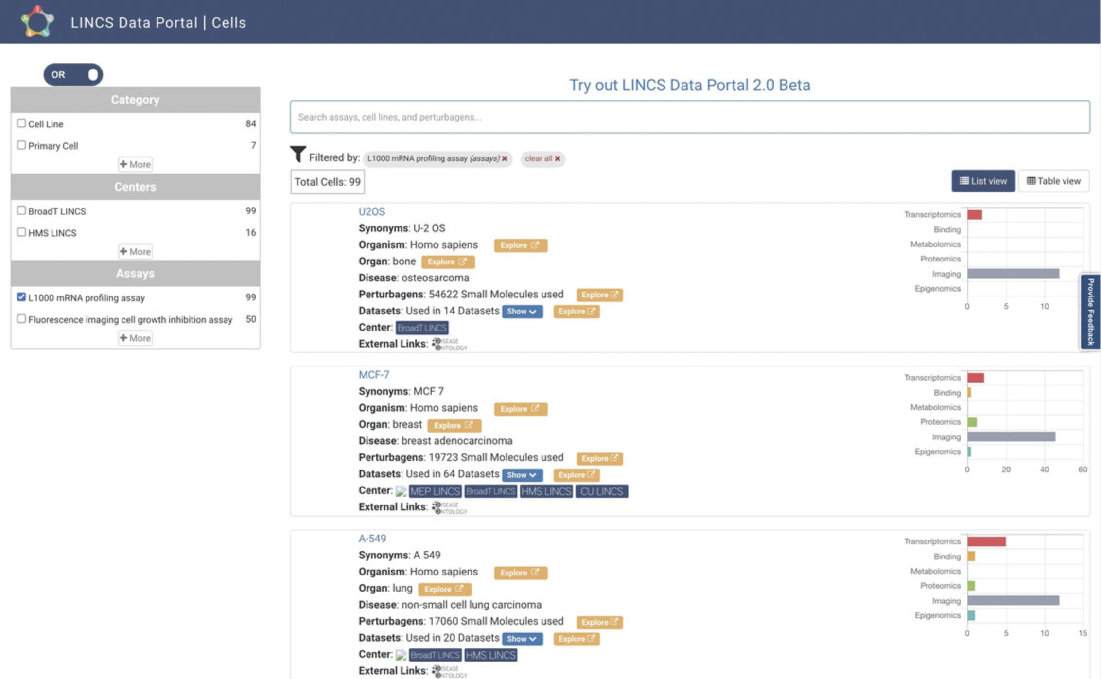
6.Starting from step 2, with the L1000 data having been selected on the homepage, click the Cells icon on the homepage. This will navigate to a cell-centric view of the L1000 data (Fig. 82). The results are displayed in Table View by default, and List View can alternatively be selected via the button above the results display. Each result lists the cell line's name; its synonyms, associated organism, organ, and disease; perturbagens that have been applied to the cell line; associated L1000 datasets; LINCS Centers that generated the associated data; and external links. A bar plot for each result displays the experimental platforms of the datasets with which that cell line is associated. Results can be searched by assays, perturbagens, and other keywords via the search box above the results display. The results can also be filtered by the type of cell, LINCS Center that generated the associated data, tissue, disease, and assay, using the menu on the left bar. Clicking on the blue “Show” button will expand the list of datasets associated with each result and provide a hyperlink to each.
Viewing the L1000 datasets from a gene perspective
7.Starting from step 2, with the L1000 data having been selected on the homepage, click the Genes icon on the homepage. This will navigate to a Harmonizome (Rouillard et al., 2016) query page that includes all the genes profiled by the L1000 assay (Fig. 83).

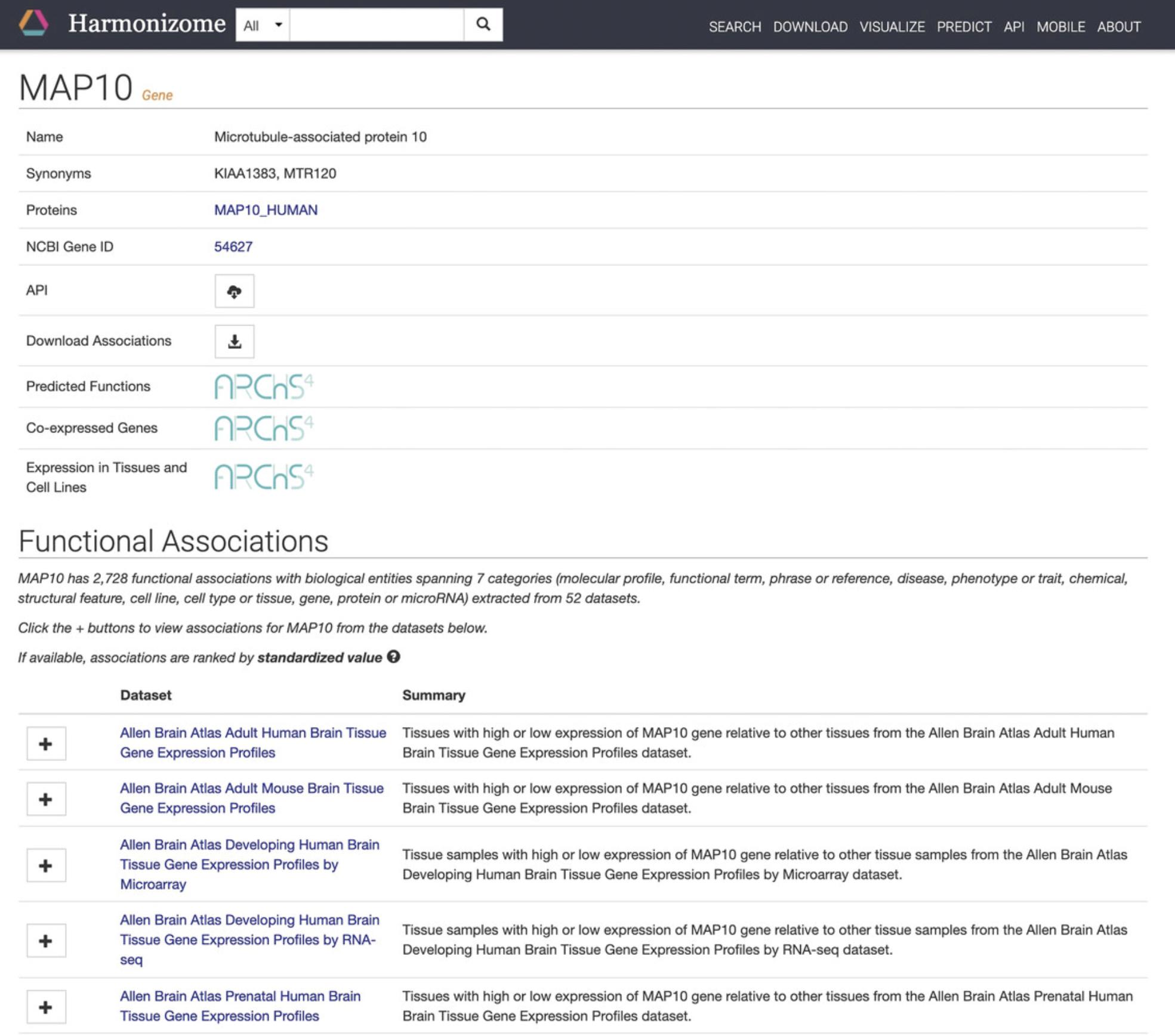
8.Click on any of the genes to be redirected to a single gene landing page with identifying metadata and functional associations for the specific gene (Fig. 84)
Using LINCS Data Portal Version 2
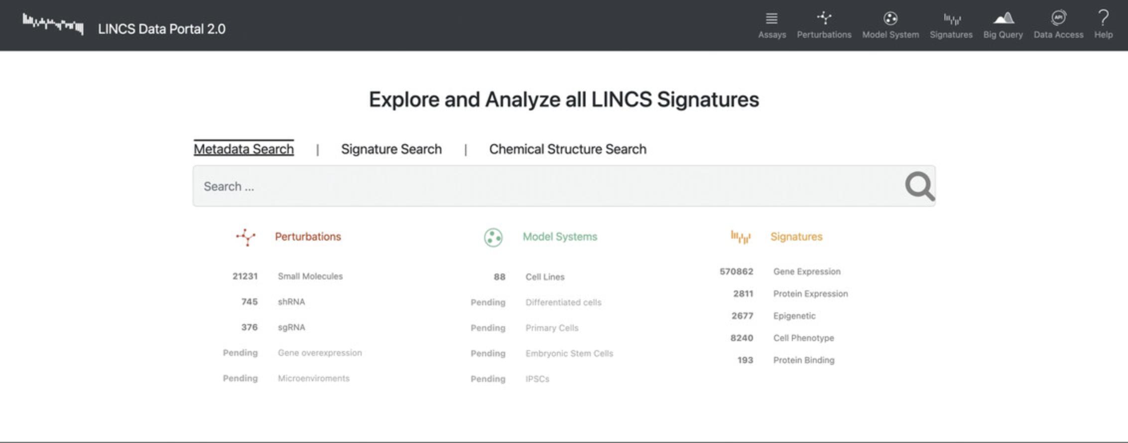
9.Navigate to the LINCS Data Portal 2.0 website (http://lincsportal.ccs.miami.edu/signatures/home; Fig. 85).
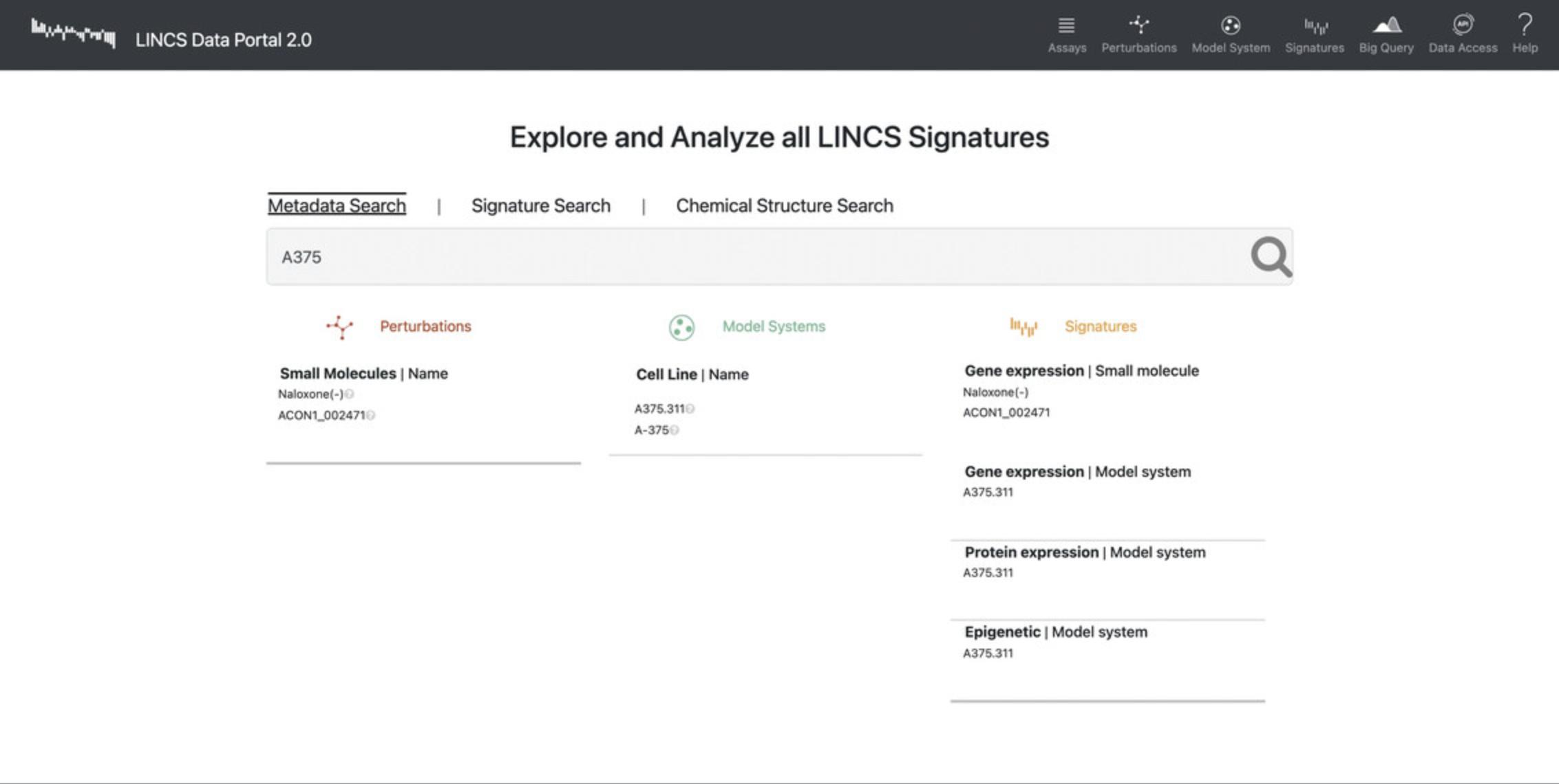
10.Select the “Metadata Search” and type in a query term of interest (i.e., A375).
Signature search
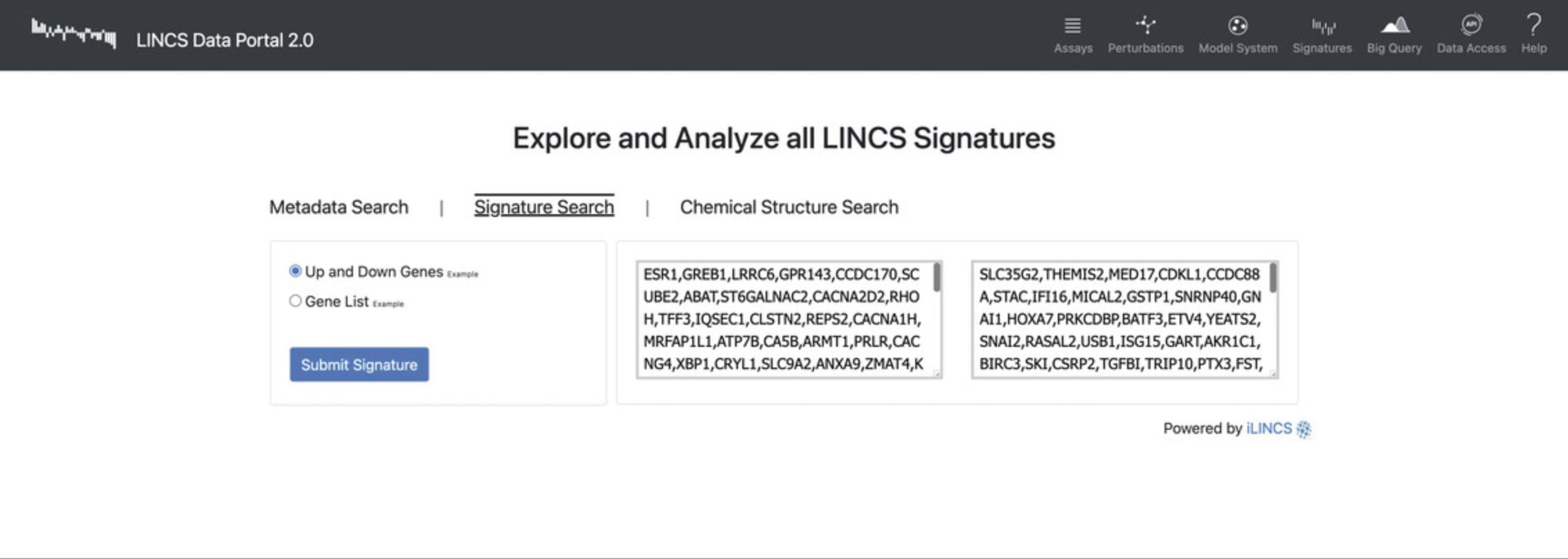
11.Select the “Signature Search” option and query an up-regulated and down-regulated set of genes, or click the “Example” text to populate the search boxes with example sets of genes (Fig. 87). Click “Submit Signature” to be redirected to a results page.
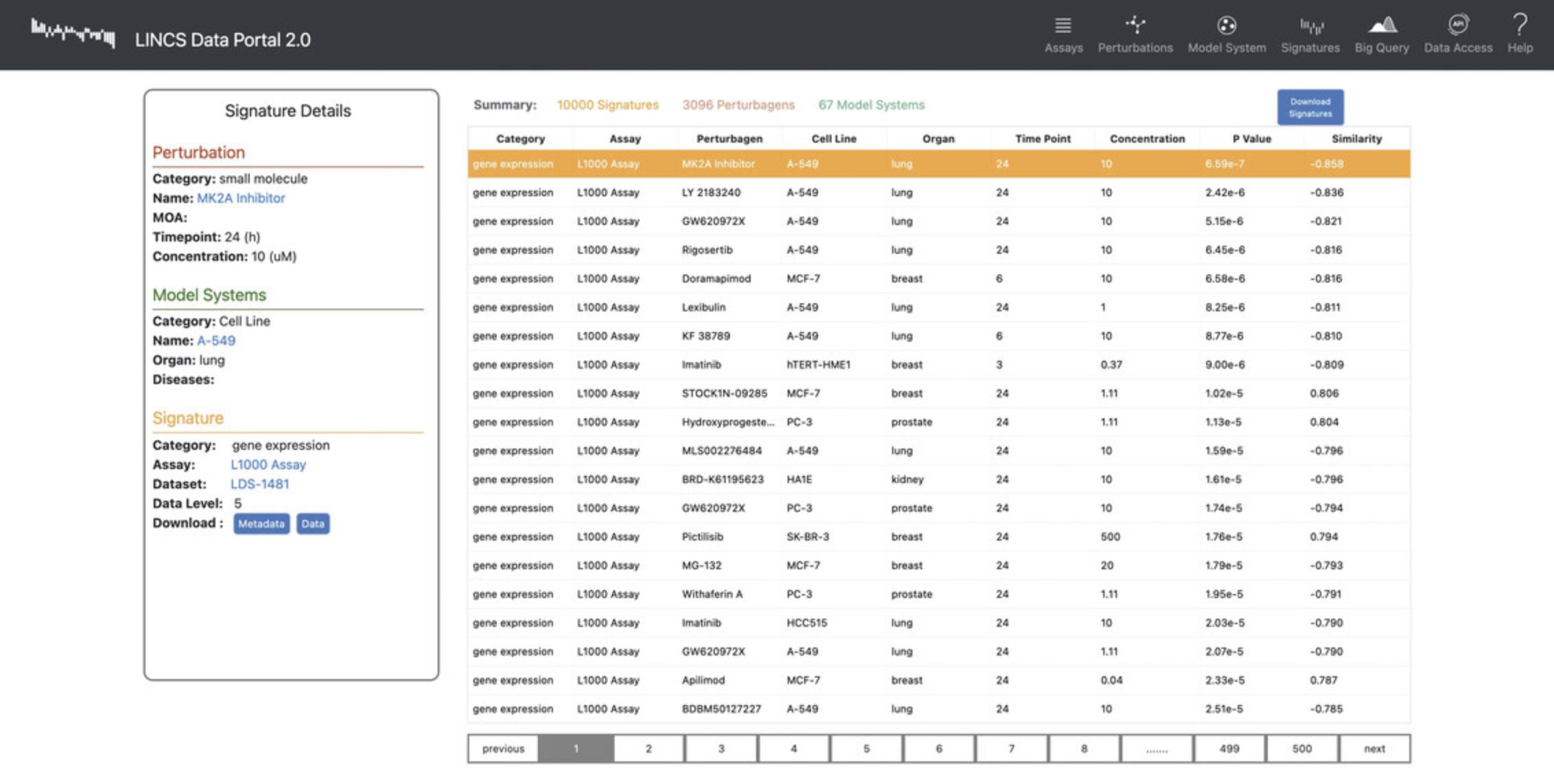
12.The results page for the signature search displays a table of the most similar and dissimilar signatures to the input, ranked by the absolute similarity values. Additionally, each signature row contains metadata about the signature including assay, perturbagen, cell line, organ, time point, and concentration (Fig. 88). Click the “Download Signatures” button to download the table.
Exploring available data in the LINCS Data Portal Version 2
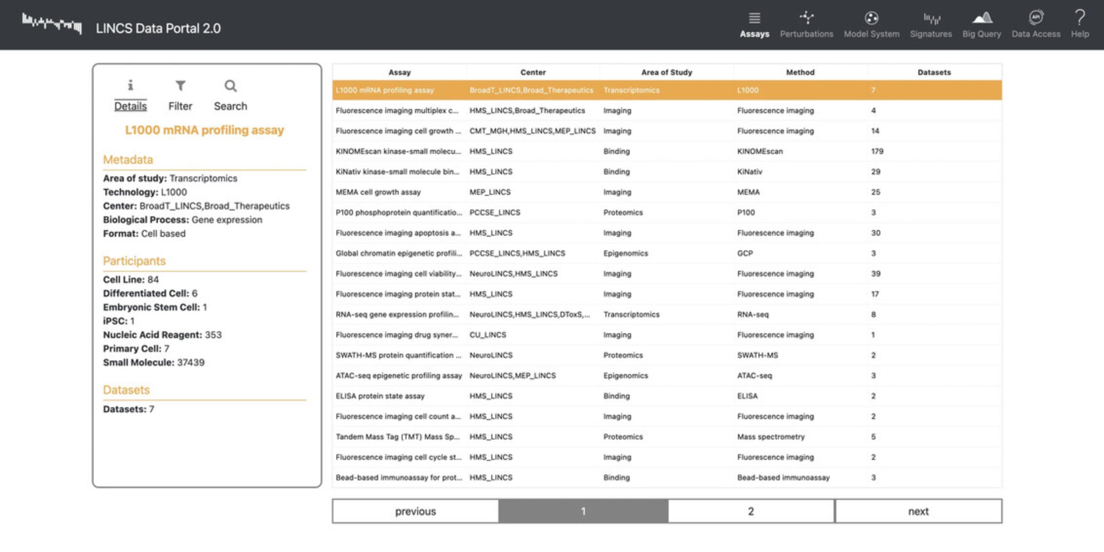
13.Click “Assays” in the navigation bar to view a list view of the assays used to generate gene expression signatures, the data generating center, the area of study, the assay method, and the number of datasets available (Fig. 89).
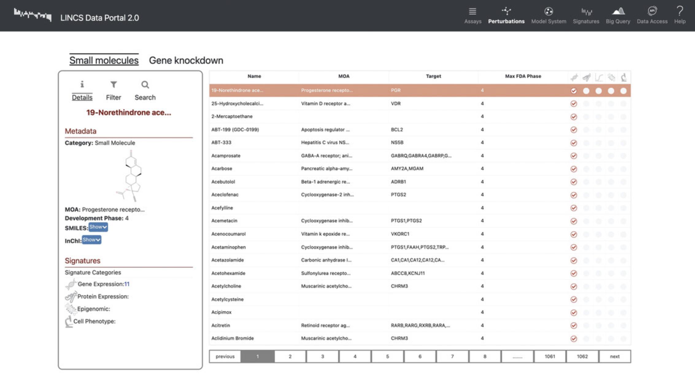
14.Click “Perturbations” in the navigation bar to be redirected to a list view of small molecules that were screened for their effect on gene expression (Fig. 90). Each row includes the mechanism of action, target, max FDA phase, and the signature categories that are applicable to the small molecule.
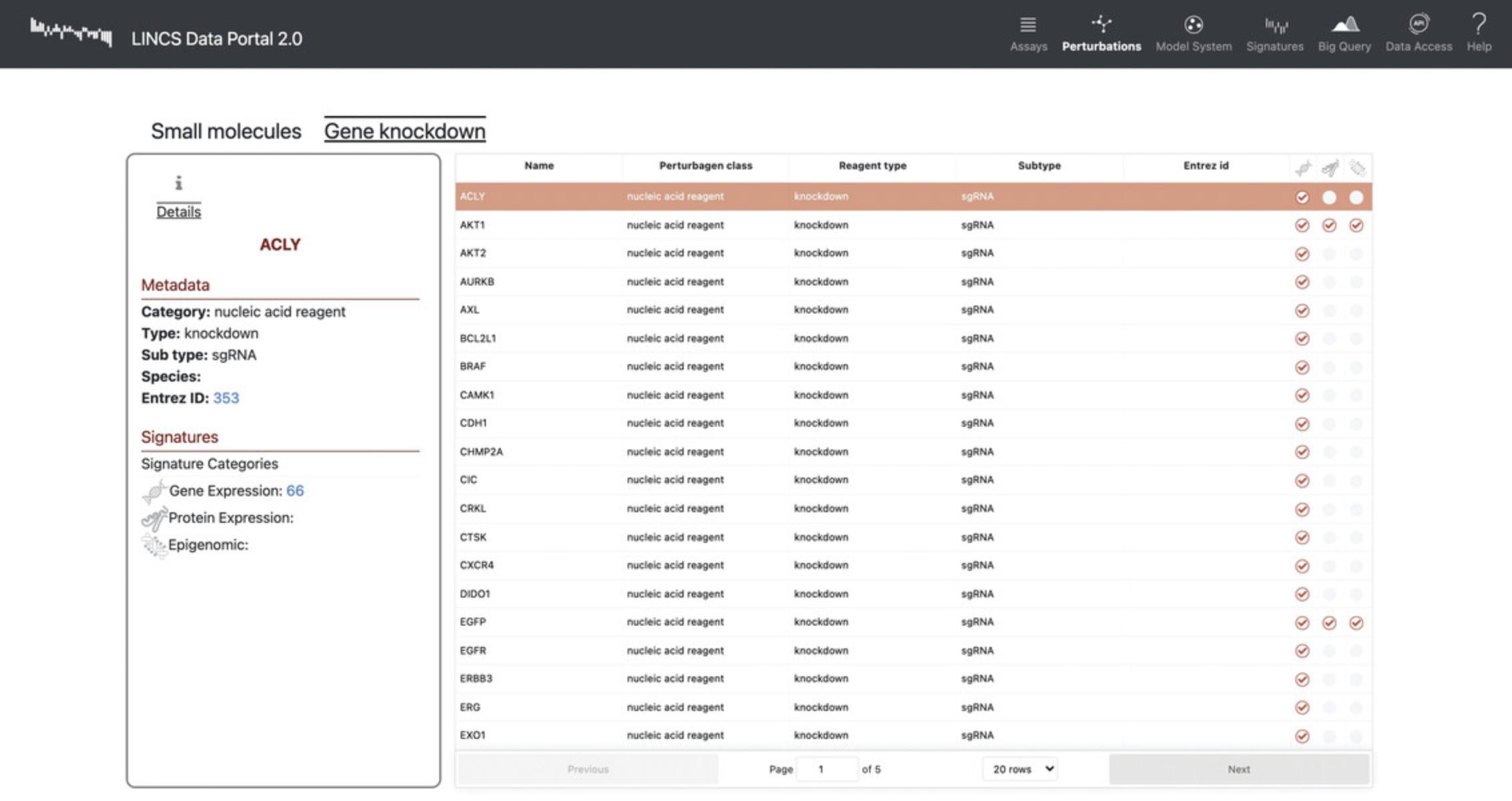
15.Click the “Gene Knockdowns” subtab on the “Perturbations” page to view a list of genes that were targeted with sgRNA to observe the effect of their knockdown on gene expression (Fig. 91). Each of the genes includes metadata regarding the perturbagen class, reagent type, subtype, and Entrez ID.
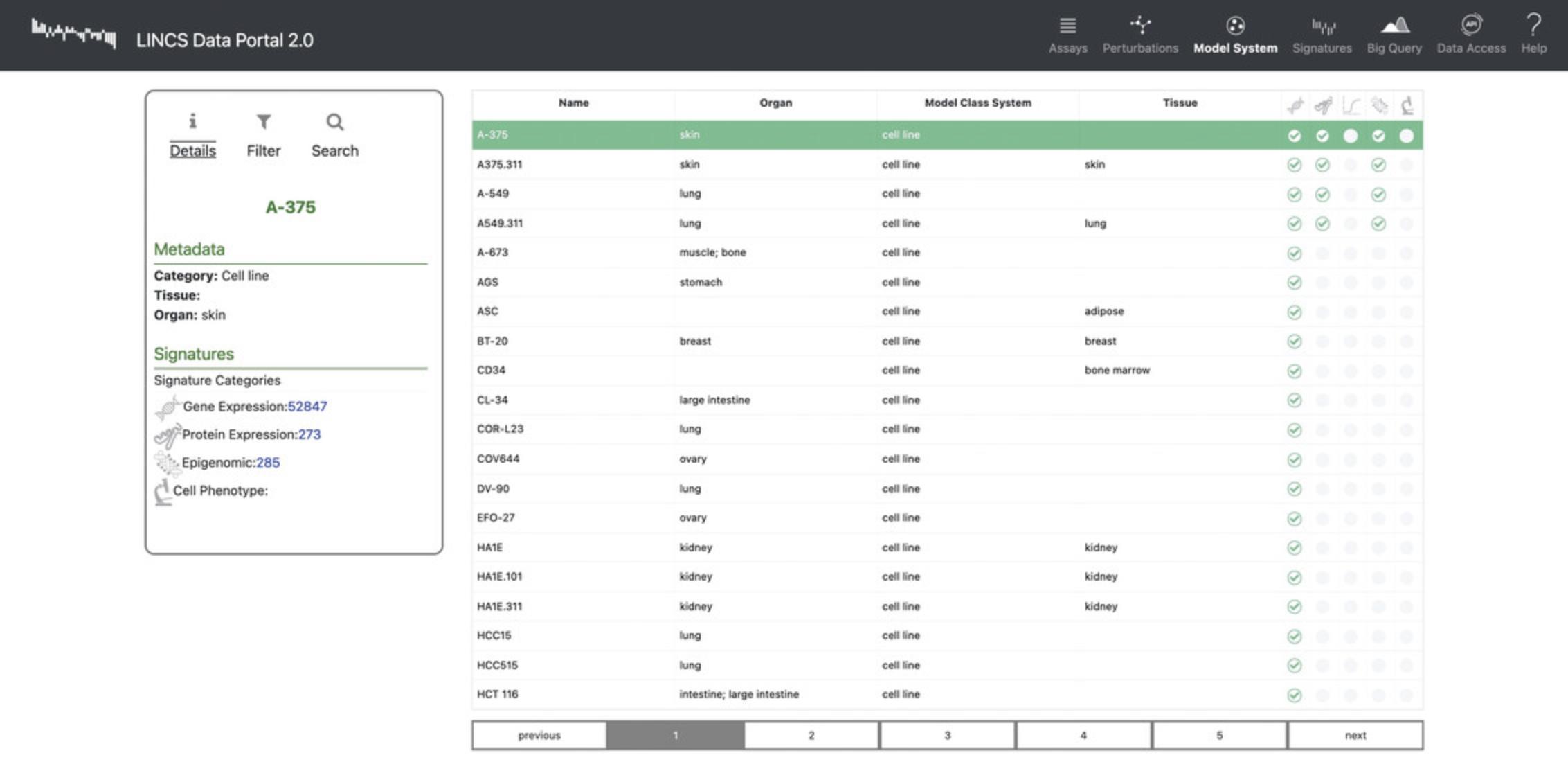
16.Click “Model Systems” in the navigation bar to view a list of cell lines that were profiled in the assays (Fig. 92). Each row includes metadata for the cell lines including organ, model class system, and tissue of origin.
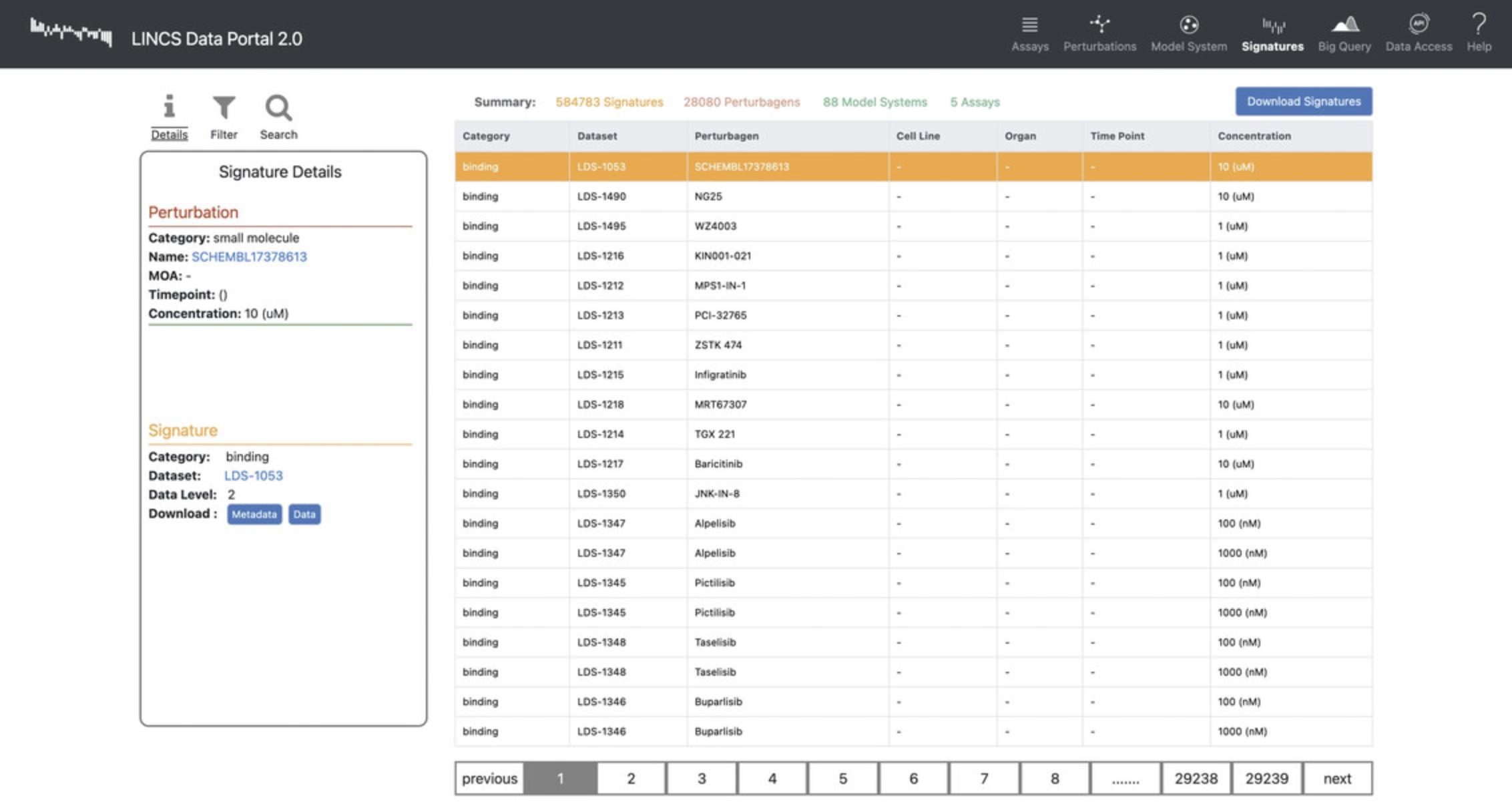
17.Click “Signatures” in the navigation bar to view all available signatures and metadata that includes the perturbation category, dataset of origin, perturbagen, cell line, organ, time point, and concentration (Fig. 93).
Using SigCom LINCS
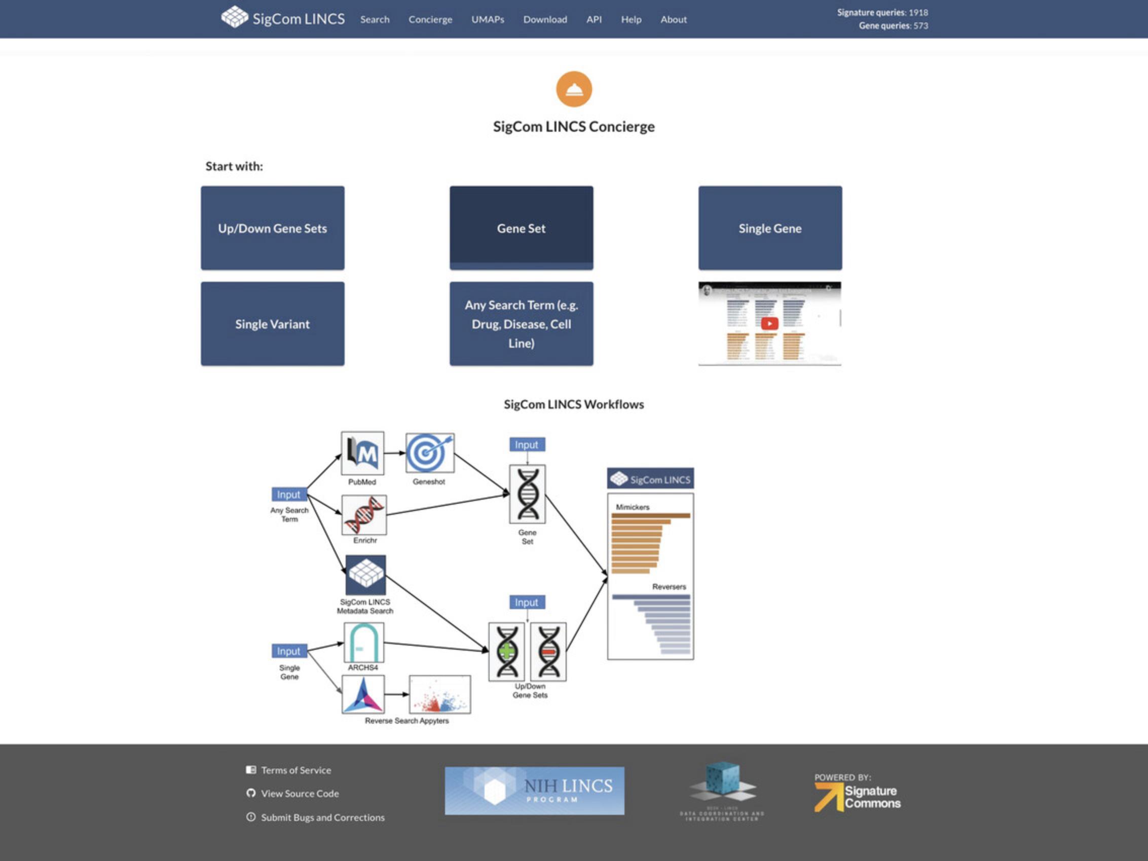
18.Navigate to the SigCom LINCS homepage at https://maayanlab.cloud/sigcom-lincs (Fig. 94).
Performing signature search enrichment analysis
19.Select the “Up/Down Gene Sets” button, then enter up-regulated and down-regulated gene names into the respective input boxes (Fig. 95). Each gene should be on its own row. The upper right-hand corner of each input box will display how many gene symbols are valid. To fix the names of genes with invalid entries, toggle the “Validate” option in the upper left-hand corner of each input box. You will be presented with all the symbols that are valid and suggestions to fix entries based on synonyms.
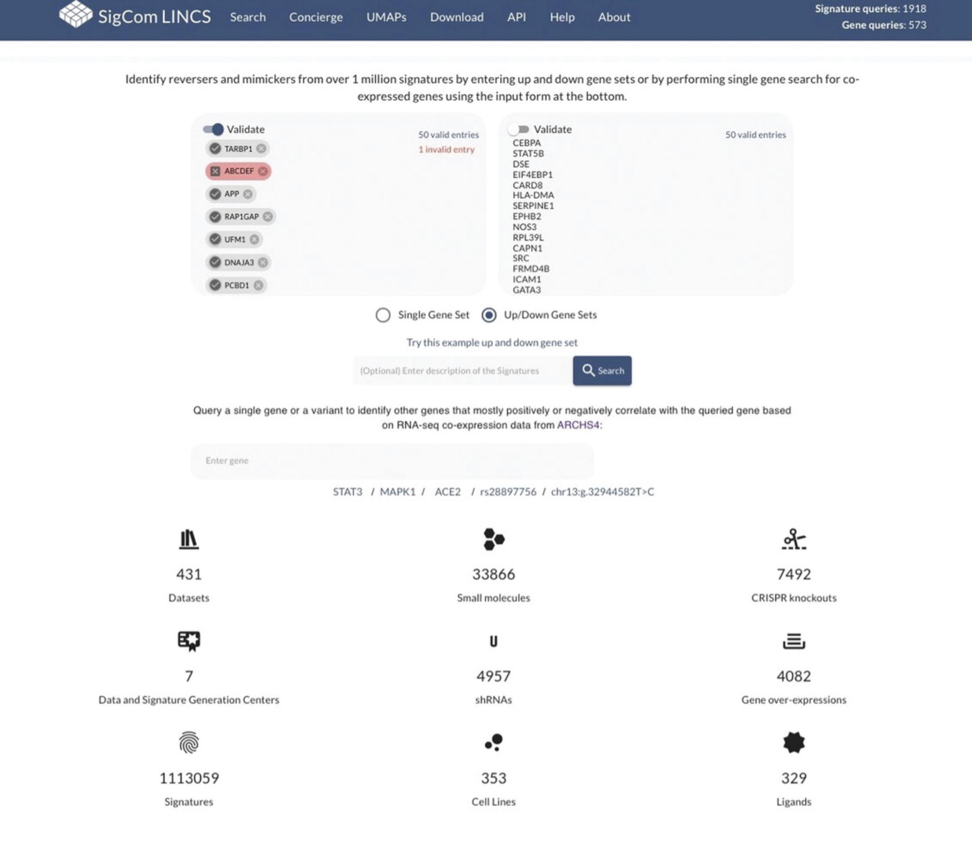
20.Click the dark blue “Search” button below the input boxes.
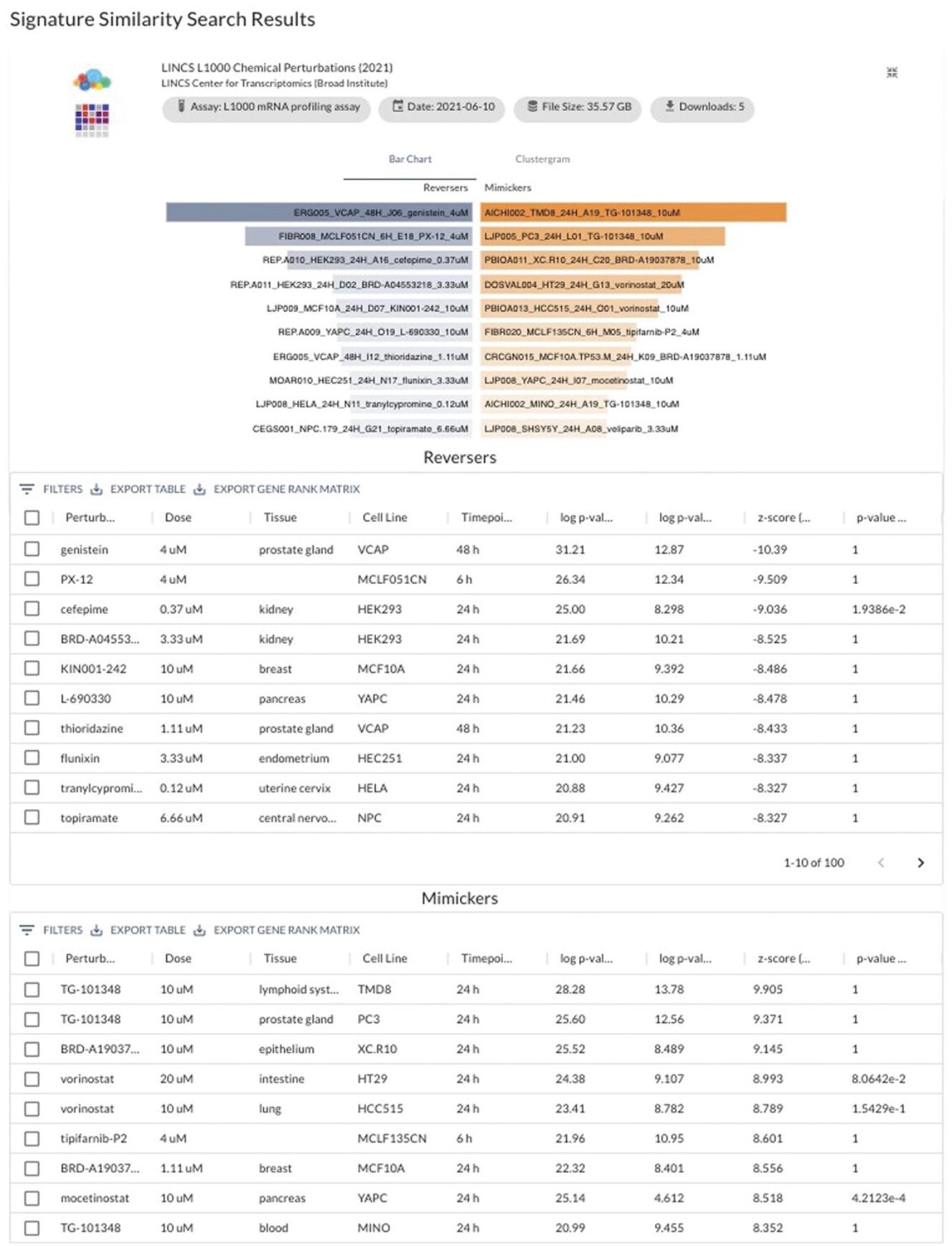
21.The top signature results for the input will be displayed separately by dataset (Fig. 96). Blue bars indicate reverser/opposite signatures, while orange bars indicate mimicker/similar signatures. Higher rank position, longer bar length, and darker color indicate results with greater significance. Hover over any bar to view the z- score generated from the Fisher Exact Test for the corresponding signature when compared to the input.
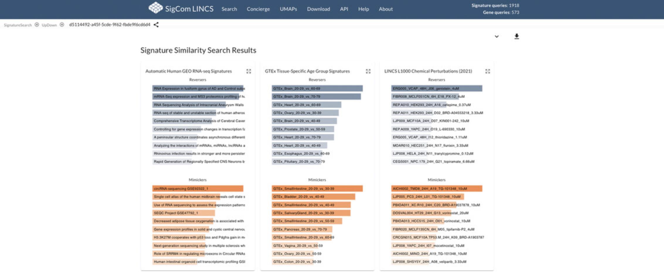
22.Click the expand icon on any of the perturbation types to view more detailed results. As an example, expand the “LINCS L1000 Chemical Perturbations” results.
- a.The “Bar Chart” detailed view tab (Fig. 97) provides a larger view of the bar charts from the initial results page, as well as tables containing all computed statistical values for each of the reverser and mimicker drugs. Tables can be downloaded as a TSV file using the download icons next to the top left of the tables.
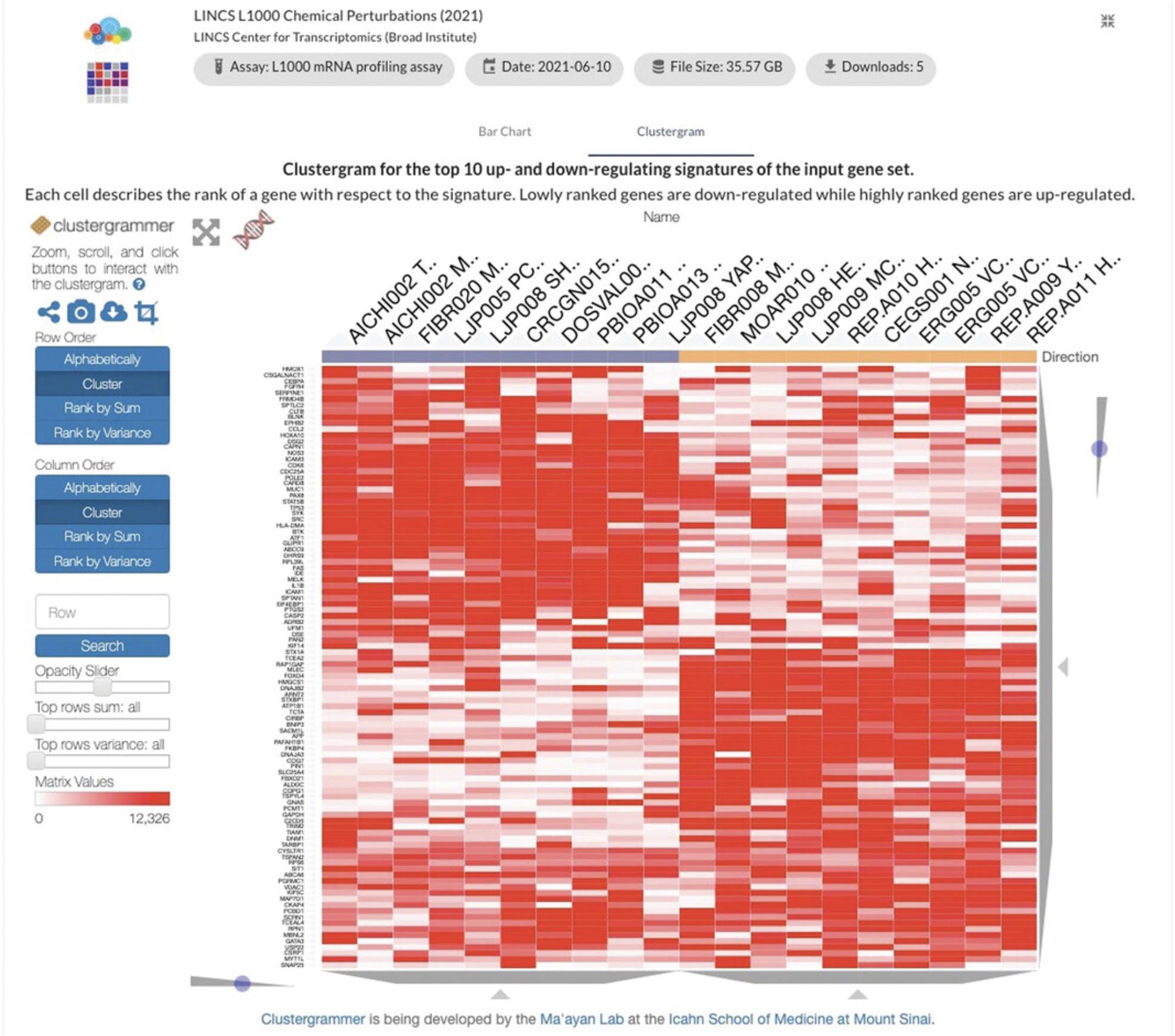
- b.The “Clustergram” detailed view tab (Fig. 98) provides a clustergram plot showing the top 10 signatures in which the input genes are most up-regulated and most down-regulated. The plot can be adjusted using the toolbar to the left. Hovering over a cell in the clustergram shows the rank of a gene (row) with respect to the given signature (column), with a low rank indicating down-regulation of the gene.
Metadata search
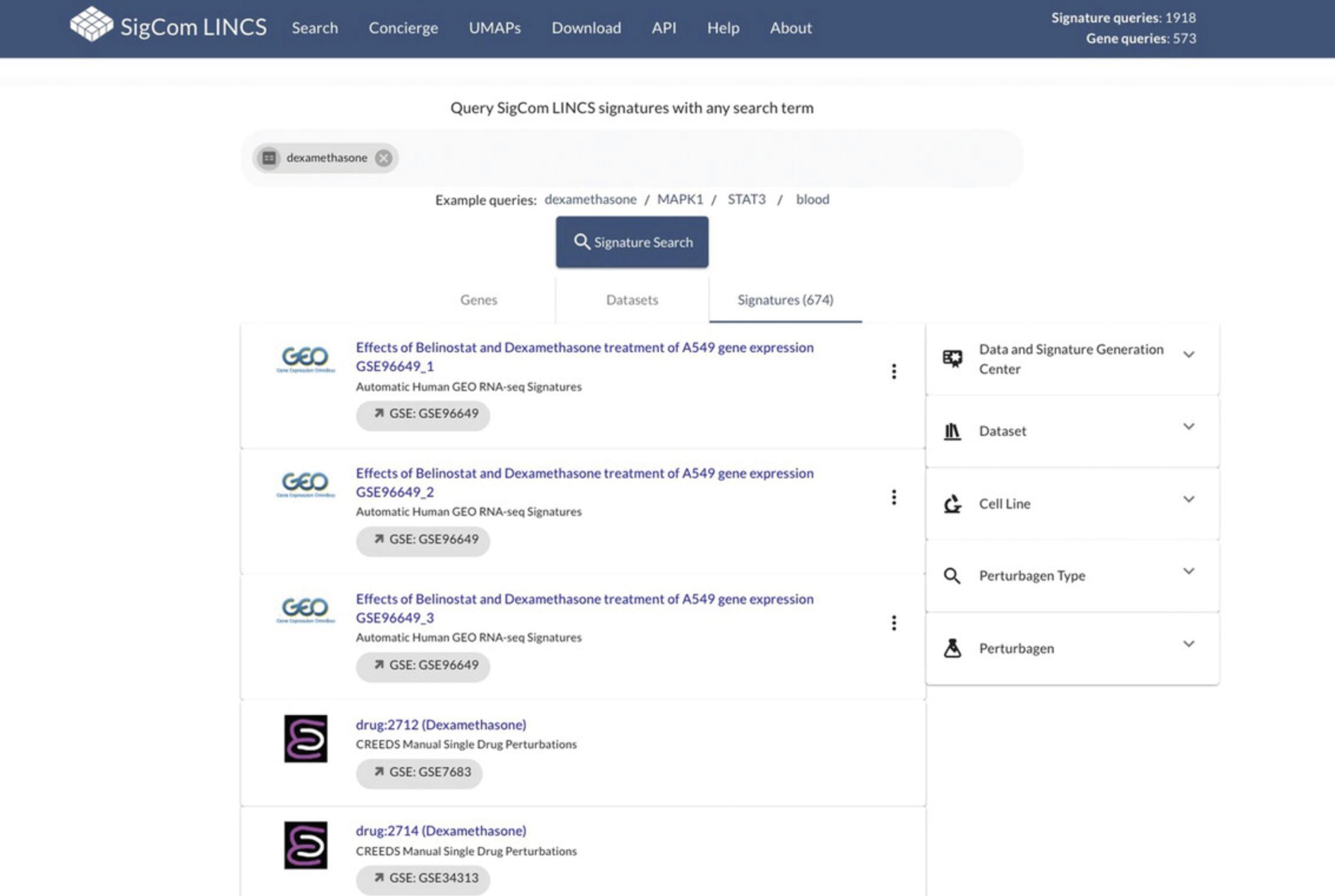
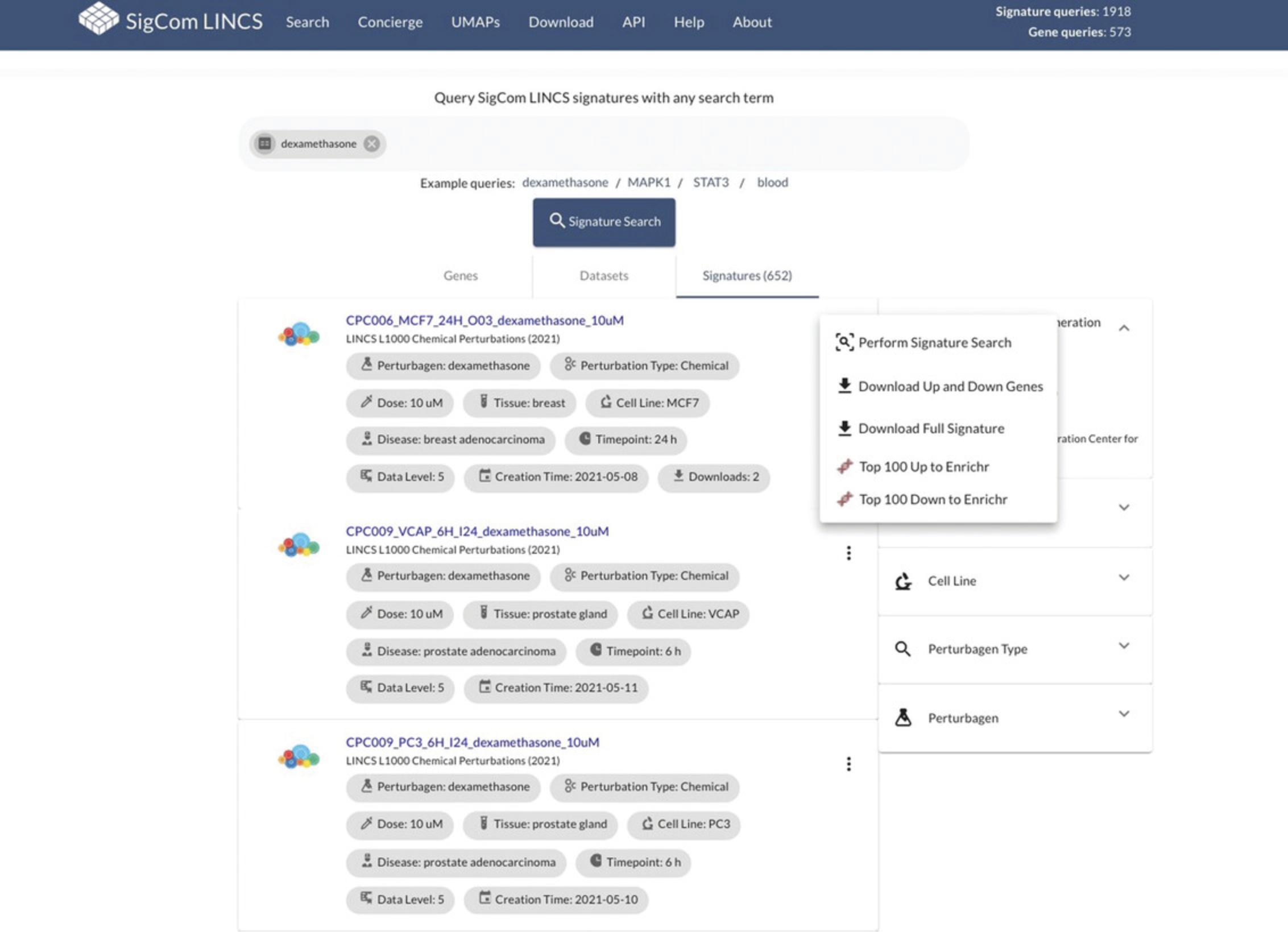
23.Select the dark blue “Any Search Term” box on the homepage (see Fig. 94), then select the orange “Perform Metadata Search” option when it appears. Enter any term of interest into the input box (disease, cellular process, drug name, gene symbol, cell line, or any other term). As an example, query the term “dexamethasone”, then select the “Signature Search” button (Fig. 99).
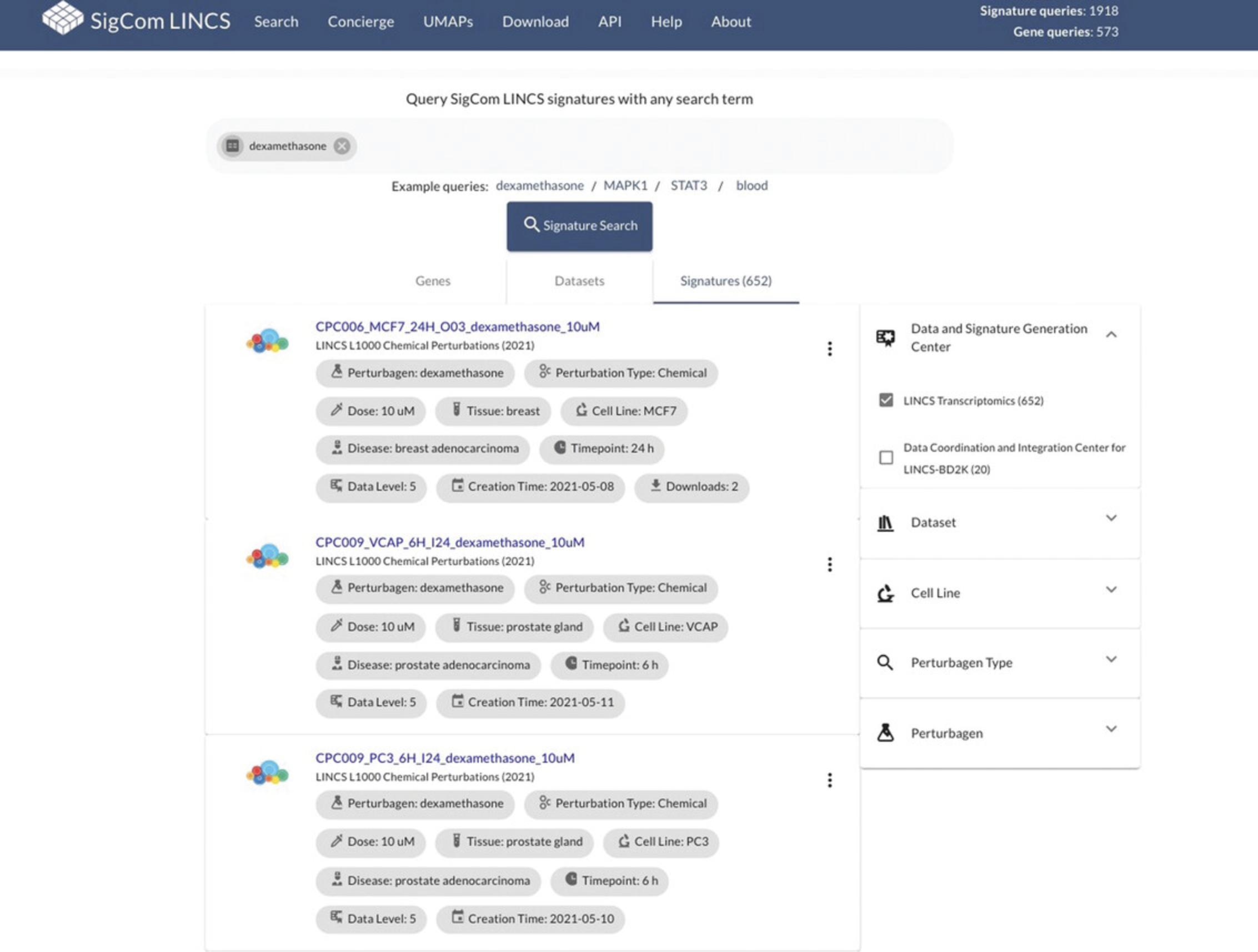
24.Select subsets of the results by choosing the “Data and Signature Generation Center”, “Dataset”, “Cell Line”, “Perturbagen Type”, or “Perturbagen” using the filter menu on the right. For example, select “LINCS Transcriptomics” under the “Data and Signature Generation Center” menu to filter returned signatures to only those generated by the LINCS Transcriptomics center (Fig. 100).
25.Click on the three dots icon to the right of each signature result (Fig. 101) to download the full signature, download the top up and down genes as a GMT file, or submit the up and down genes from that signature to the SigCom LINCS Signature Search. See steps 4-5 above to understand how to interpret the Signature Search results.
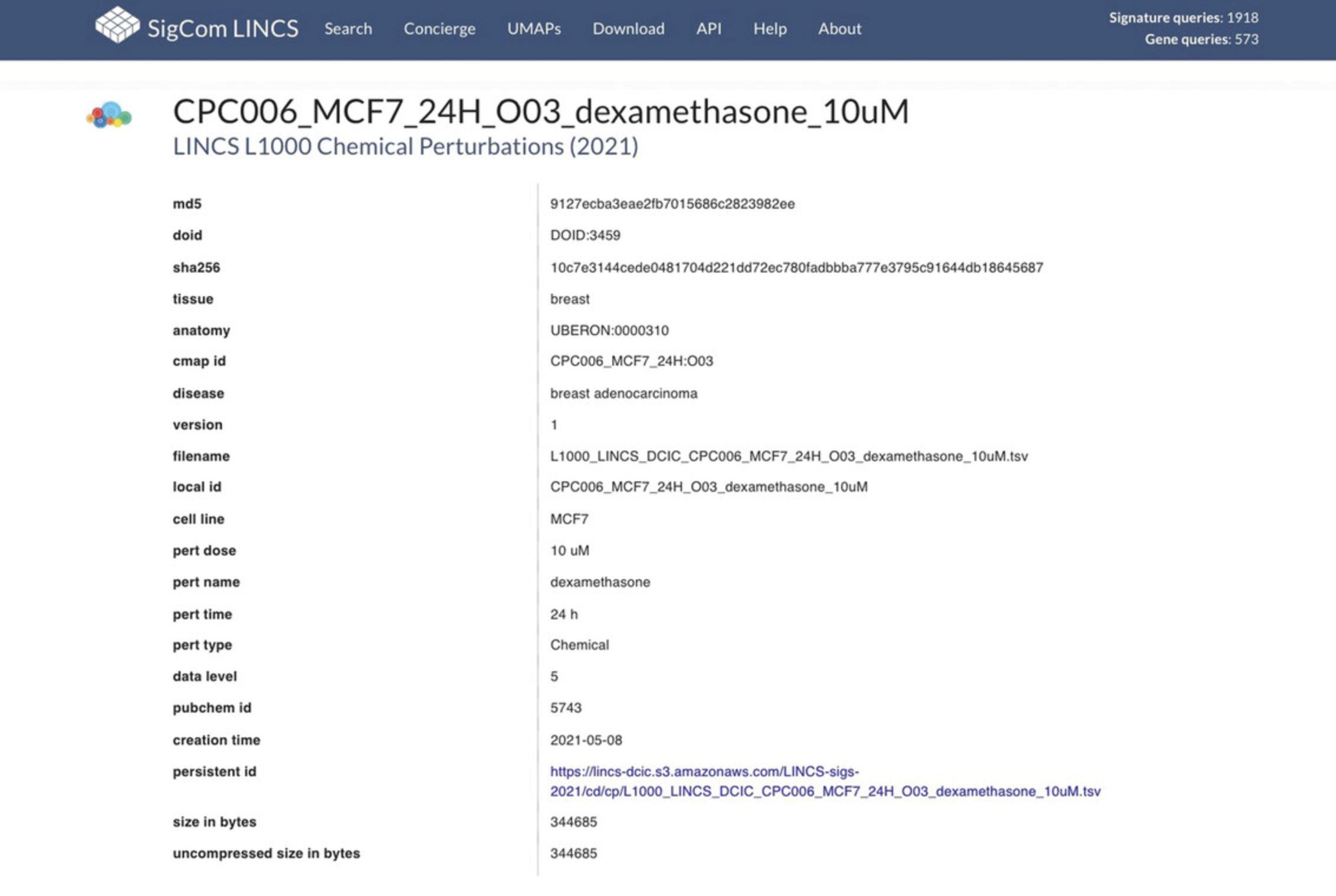
26.Click on a signature name to view detailed metadata for that signature (Fig. 102).
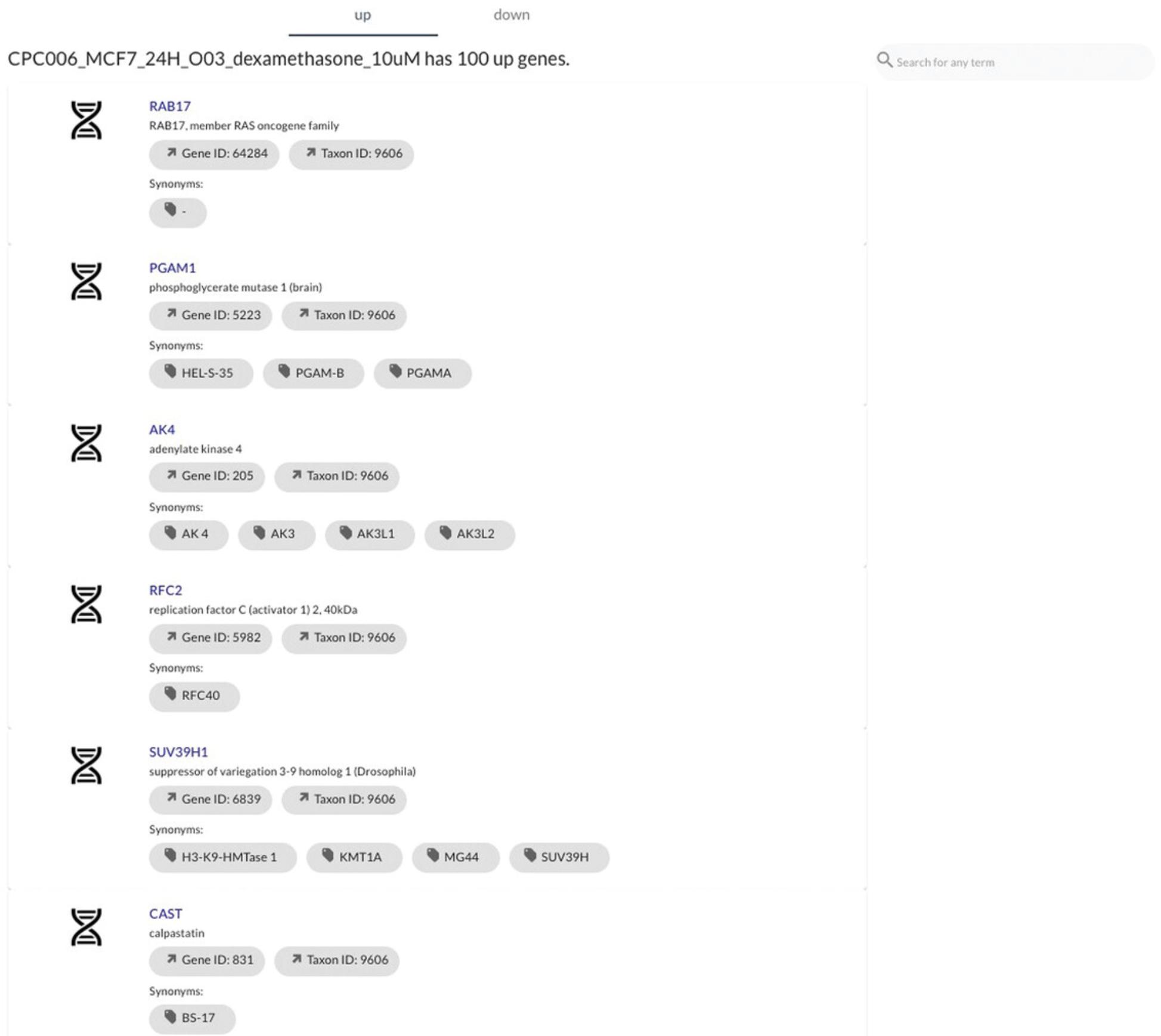
27.Scroll below the metadata information to view the top up- and down-regulated genes in the signature. By default, the up genes are shown (Fig. 103). Select the “down” tab to view down genes.
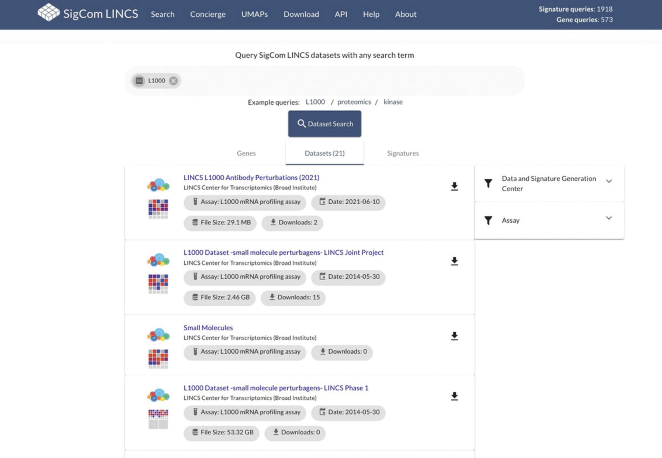
28.Return to the metadata search page by using the back button in your browser. To search through available datasets, click on the “Datasets” tab under the metadata search bar (Fig. 104). As an example, remove any existing terms in the search bar and query “L1000”. Dataset results can be sorted by Data and Signature Generation Center or Assay using the menu on the right-hand side. As an example, select “LINCS Transcriptomics” as the Data and Signature Generation Center. Hover over the FAIRshake icon for a dataset to view scores for each of the categories. Click on the download icon to download the dataset.
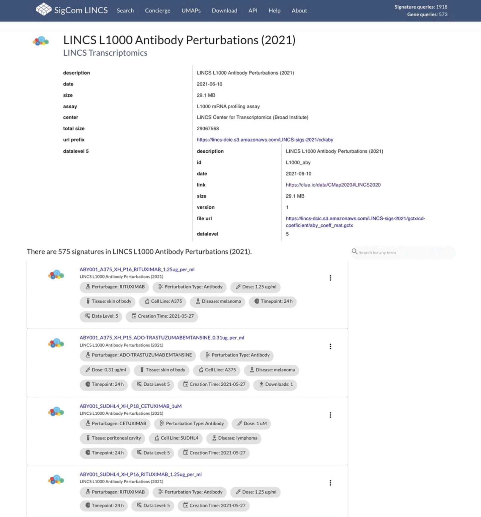
29.Click on any dataset name to view metadata for that dataset, as well as all signatures belonging to the dataset (Fig. 105).
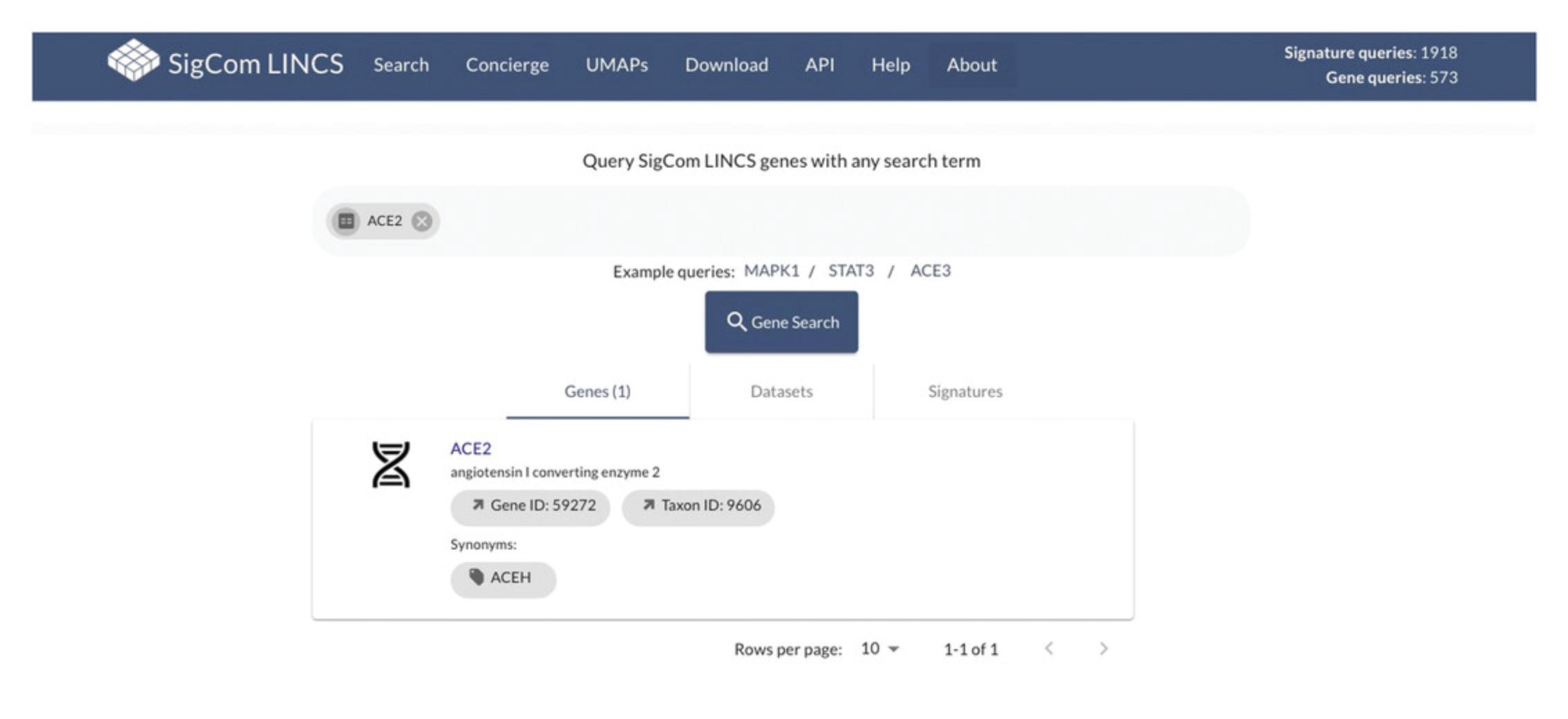
30.Return to the metadata search page by using the back button in your browser. To search for a gene, click on the “Genes” tab under the metadata search bar (Fig. 106). Remove any existing terms and enter a gene of interest, such as ACE2, in the search bar. All matching results will load automatically.
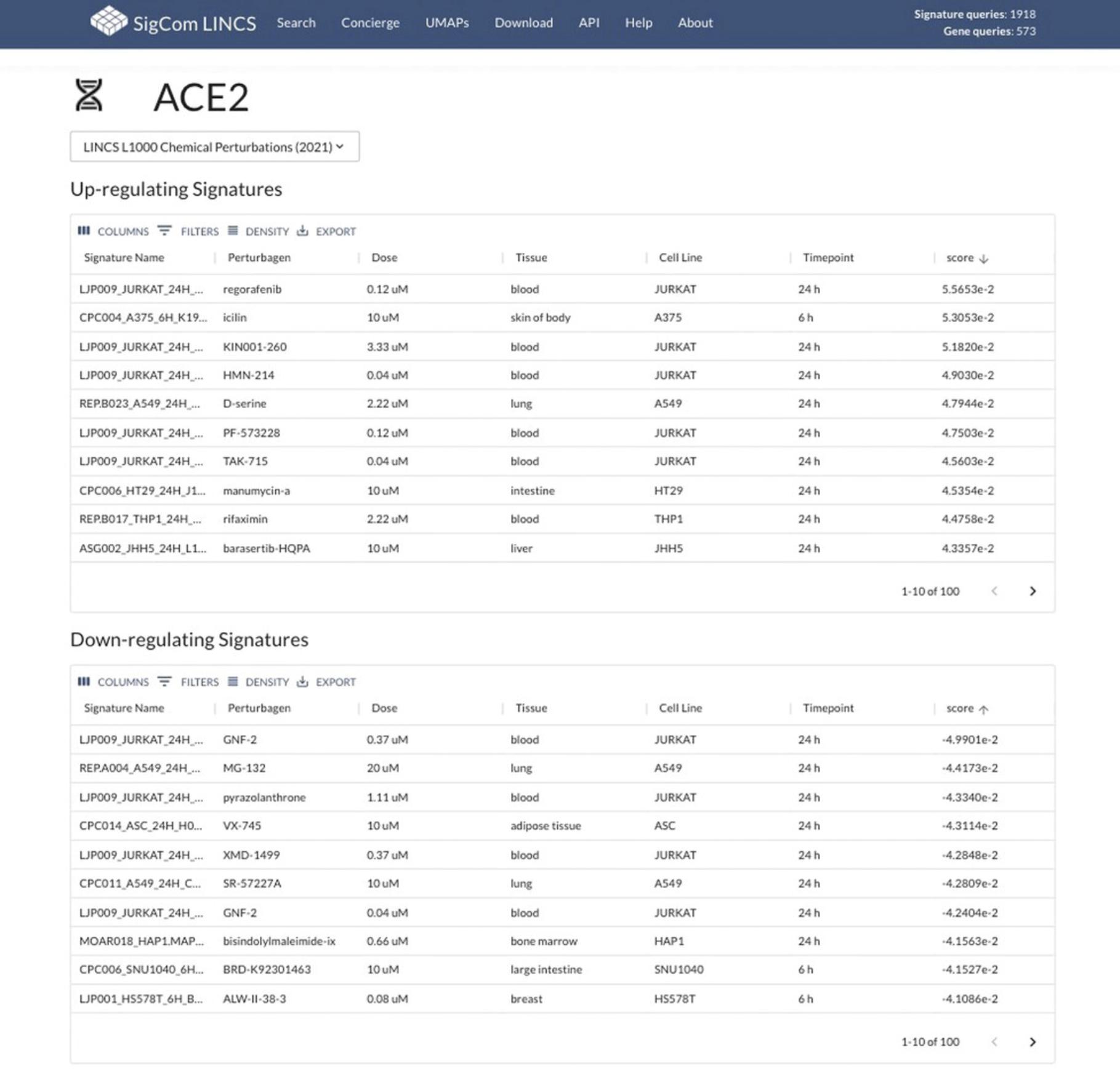
31.Click on a gene name to view signatures where the gene is significantly up-regulated or down-regulated (Fig. 107).
Visualizing SigCom LINCS signatures using UMAP
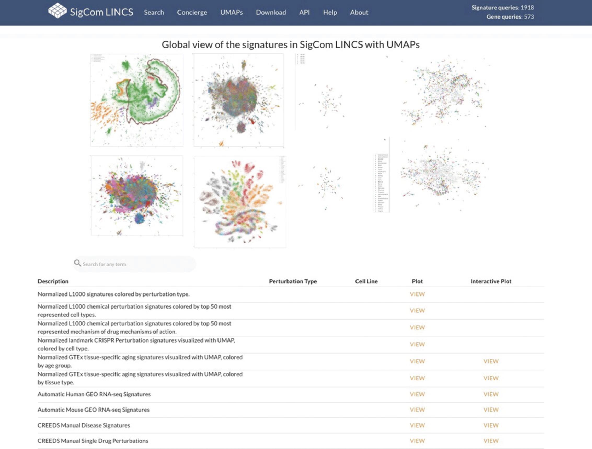
32.Click the “UMAPs” tab in the navigation bar at the top of the page. The page includes several screenshots of UMAP visualizations of various signature datasets, each of which can be selected to view a full-size visualization. Additionally, there is a table describing each dataset, associated metadata, and links that redirect to interactive and static visualizations for each dataset (Fig. 108).
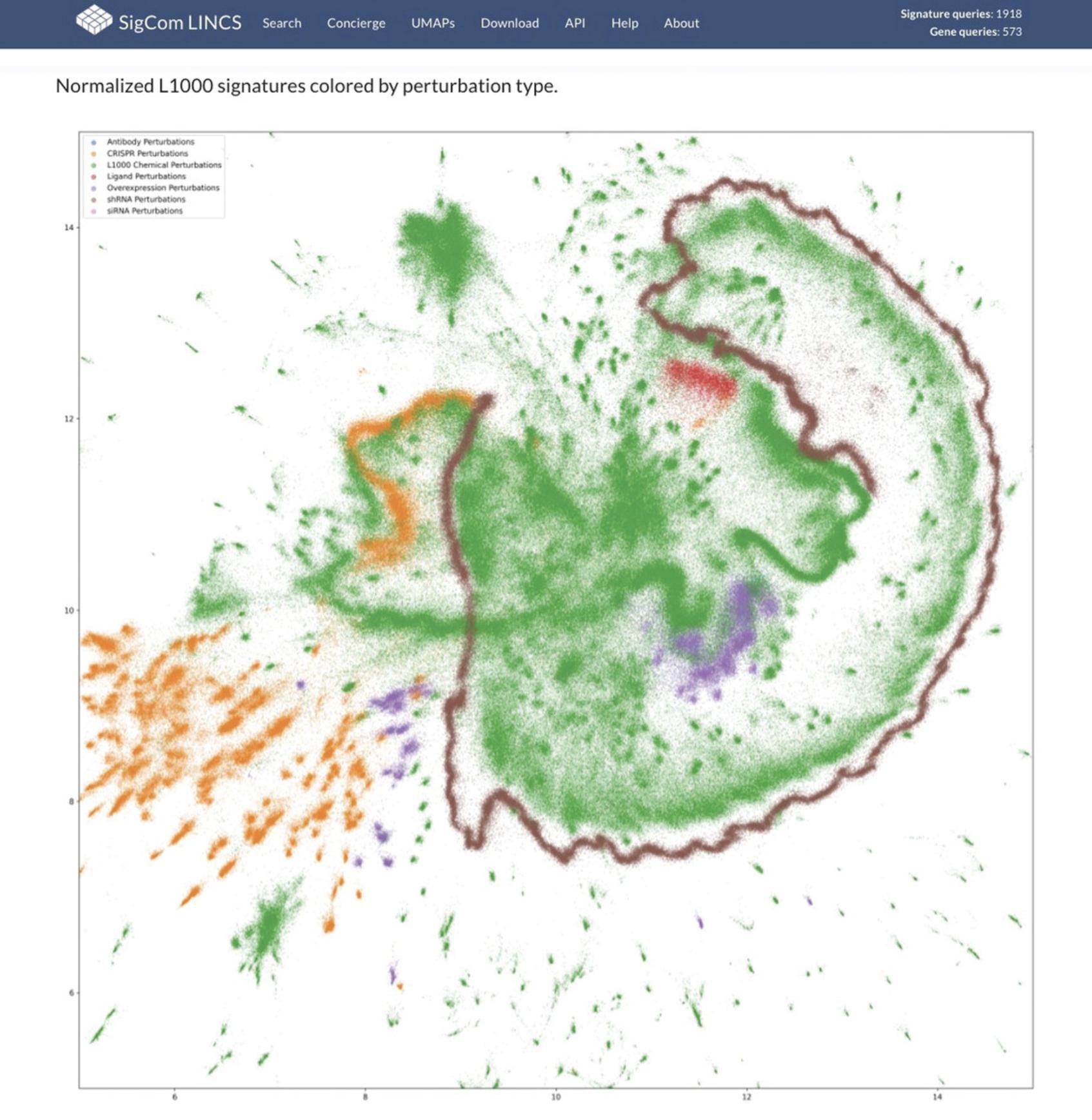
33.For an example of a static plot, click on the “VIEW” link for the “Normalized L1000 signatures colored by perturbation type” dataset in the table. The visualization is a static UMAP plot of all L1000 signatures colored by perturbation type (Fig. 109).
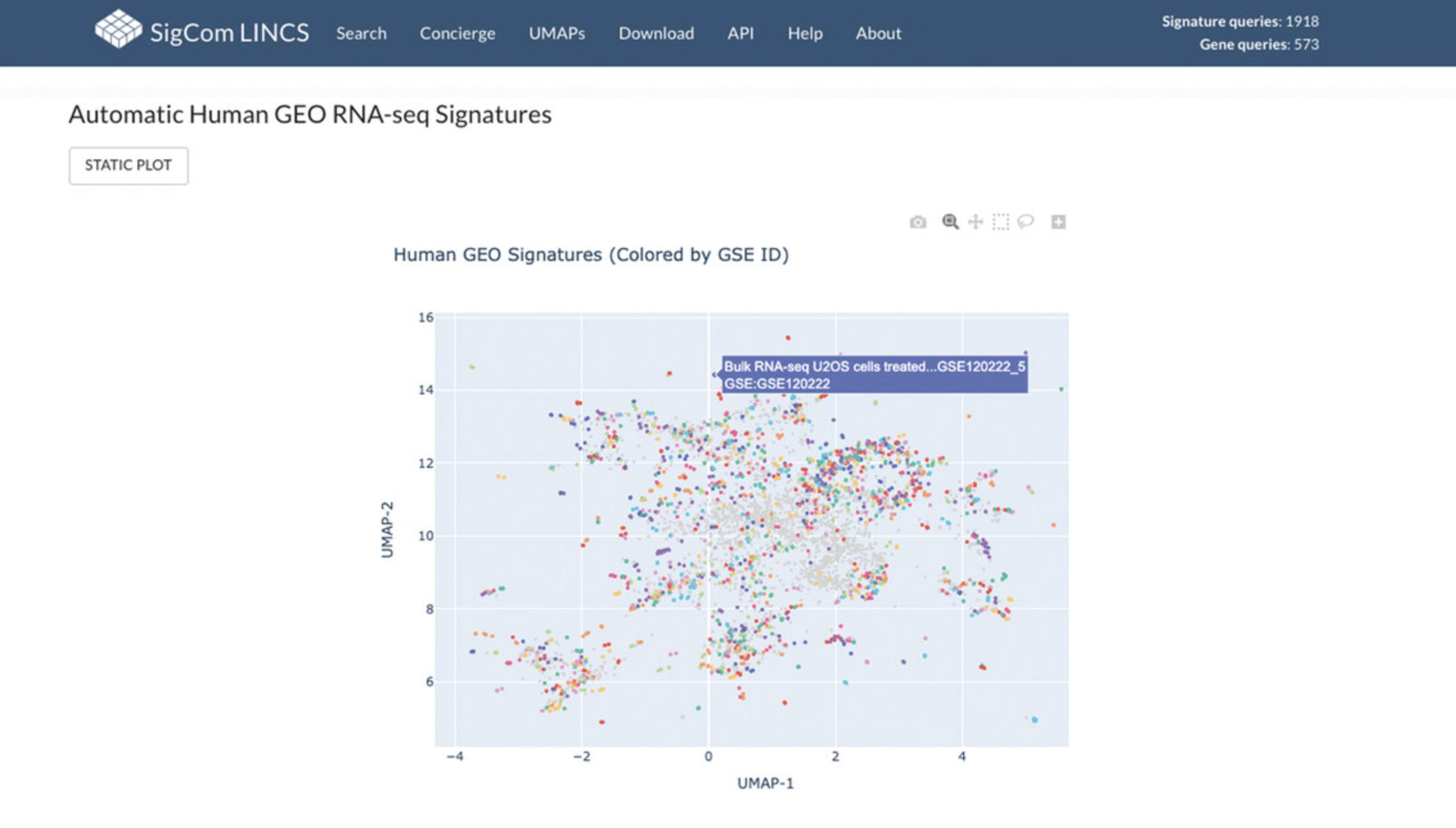
34.For an example of an interactive plot, click on the “VIEW” link in the “Interactive plot” column for the “Automatic Human GEO RNA-seq Signatures” dataset in the table. The visualization is an interactive UMAP plot where signatures are colored by GSE ID. Each point represents a signature and can be moused over for more information (Fig. 110).
Basic Protocol 9: CREATING AND ANALYZING SIGNATURES WITH iLINCS
iLINCS is a cloud-based platform maintained by the LINCS DCIC (Pilarczyk et al., 2020). iLINCS provides access to raw data and processed signatures and the ability to analyze these data using various workflows. The iLINCS portal has several user interfaces for analyzing transcriptomics and proteomics LINCS datasets. The portal integrates the R analytical engine via several R tools for web computing (rserve, opencpu, Shiny, rgl) and DCIC-developed web tools and applications (FTreeView, Enrichr, and X2K; Clarke et al., 2018) into a coherent web platform for LINCS data analysis. Users can follow several workflows that enable identifying differentially expressed genes, proteins, and phosphoproteins in LINCS datasets, and then use these signatures for analysis together with other LINCS and non-LINCS datasets, and in the analysis of LINCS L1000 signatures.
Necessary Resources
Hardware
Desktop or a laptop computer, or a mobile device, with a fast Internet connection
Software
- An up-to-date web browser such as Google Chrome (https://www.google.com/chrome/), Mozilla Firefox (https://www.mozilla.org/en-US/firefox/), Apple Safari (https://www.apple.com/safari/), or Microsoft Edge (https://www.microsoft.com/en-us/edge)
1.Navigate to the iLINCS data portal (http://www.ilincs.org/ilincs/).
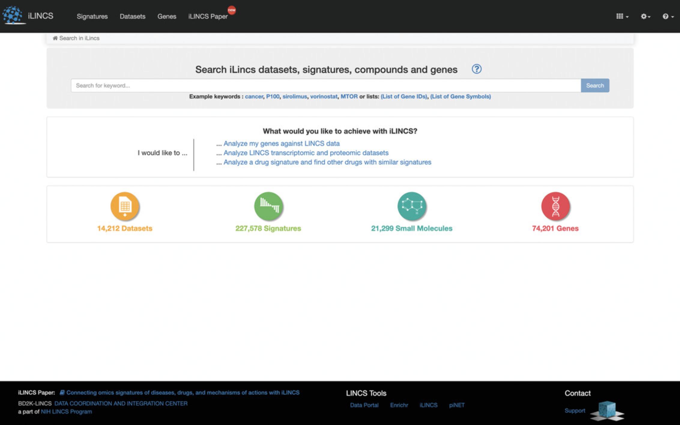
2.The homepage includes a search bar for querying search terms related to datasets, signatures, compounds, and genes found in iLINCS (Fig. 111). Type everolimus into the search field to launch a search.
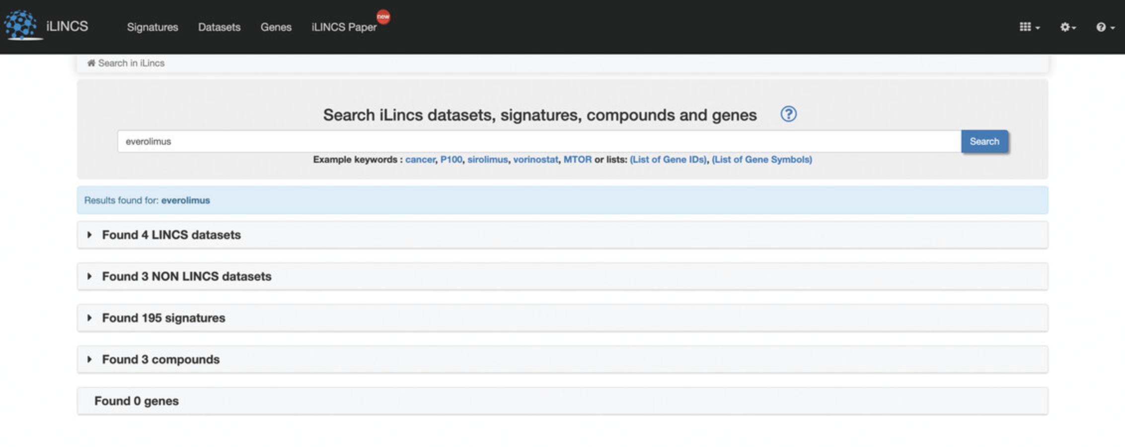
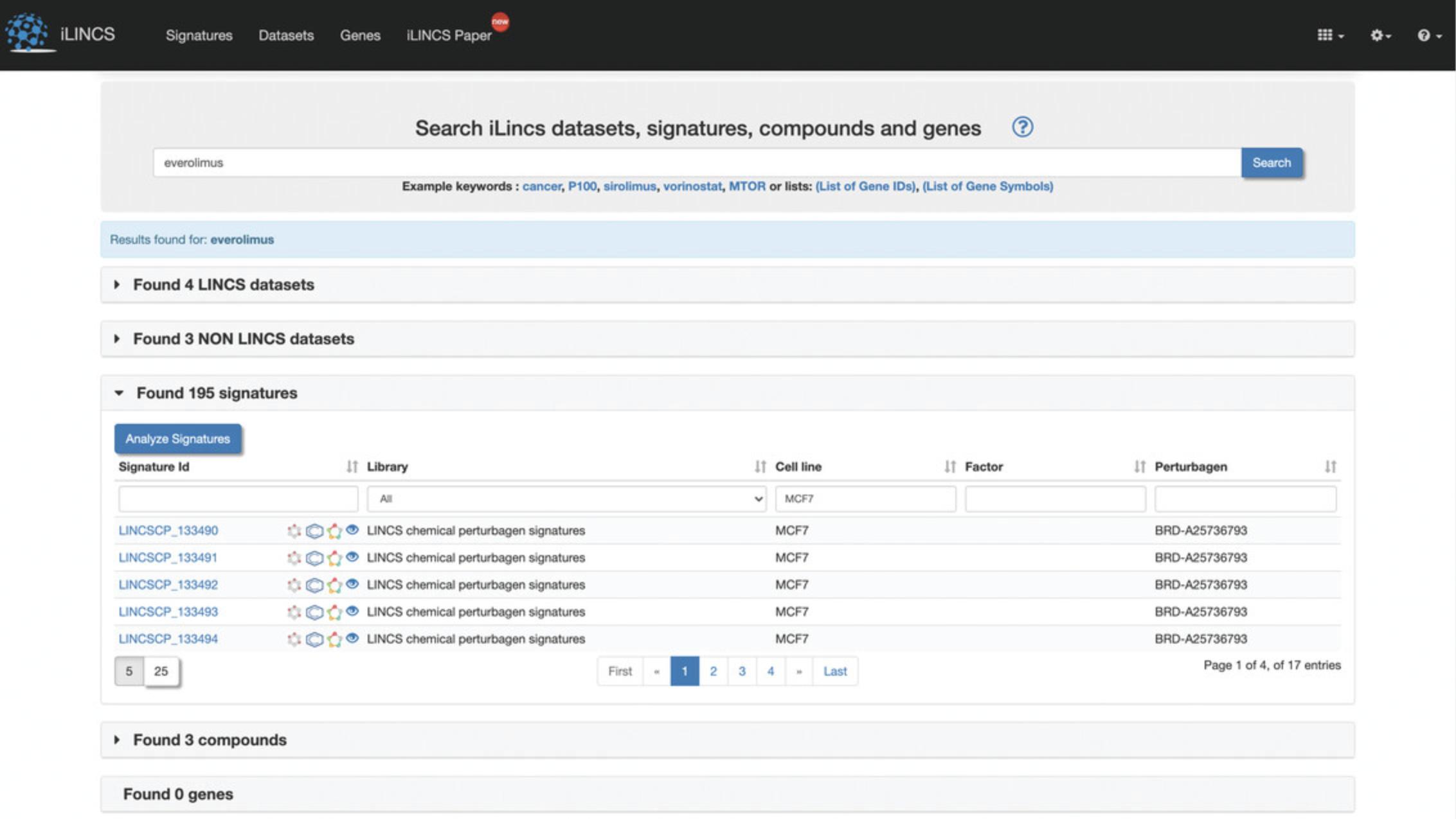
3.The results page displays LINCS datasets, non-LINCS datasets, signatures, and compounds that match everolimus (Fig. 112).
4.Expand the tab containing signatures to view a table of signatures related to “everolimus”. The table can be filtered by typing in filter keywords below each of the column headers, for example, type MCF7 below the cell line header to filter by signatures from the MCF7 cell line (Fig. 113).
Signature Details
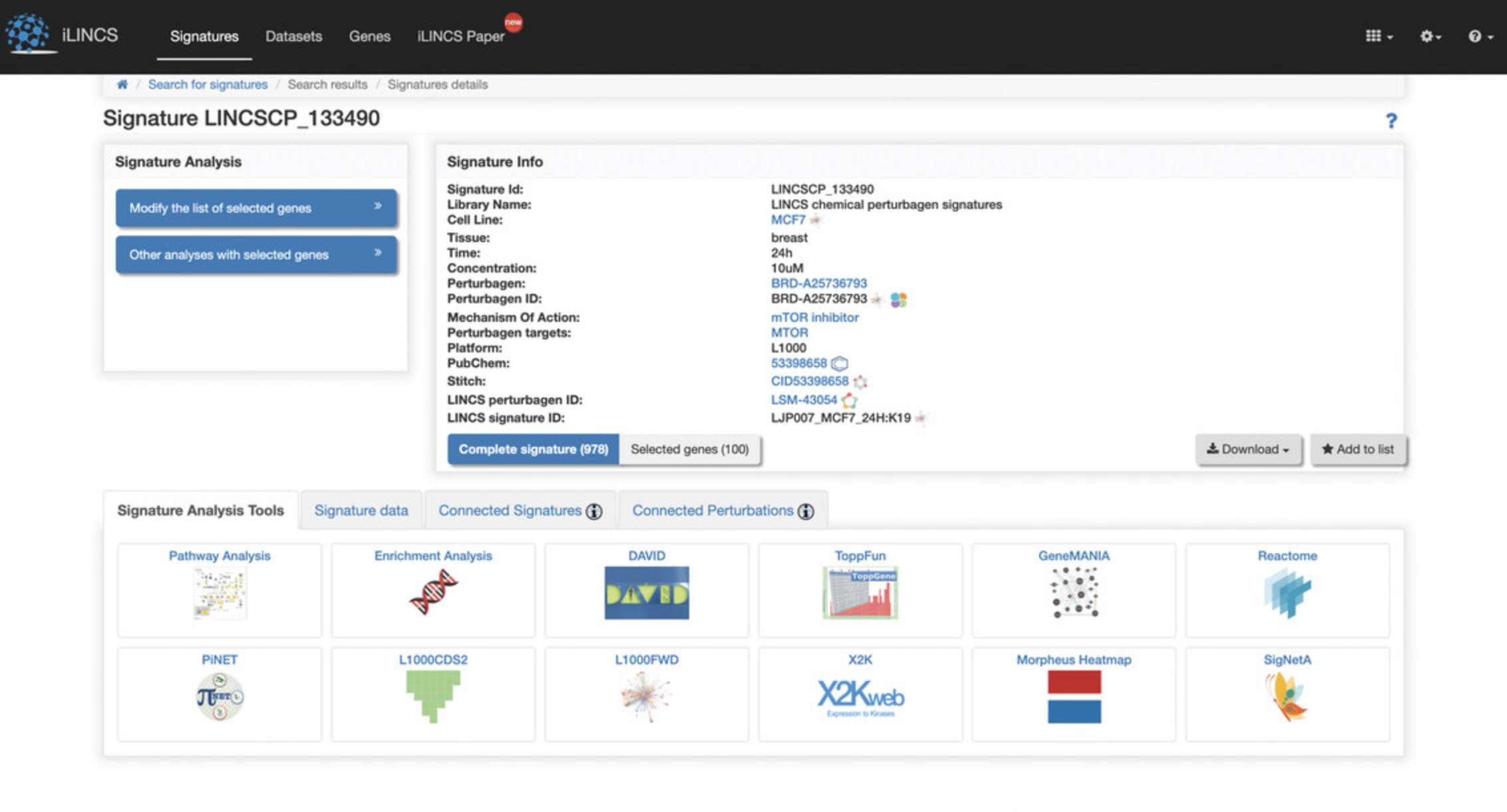
5.Click on the “LINCSCP_133490” signature within the signature id column to be redirected to a page with signature details (Fig. 114).
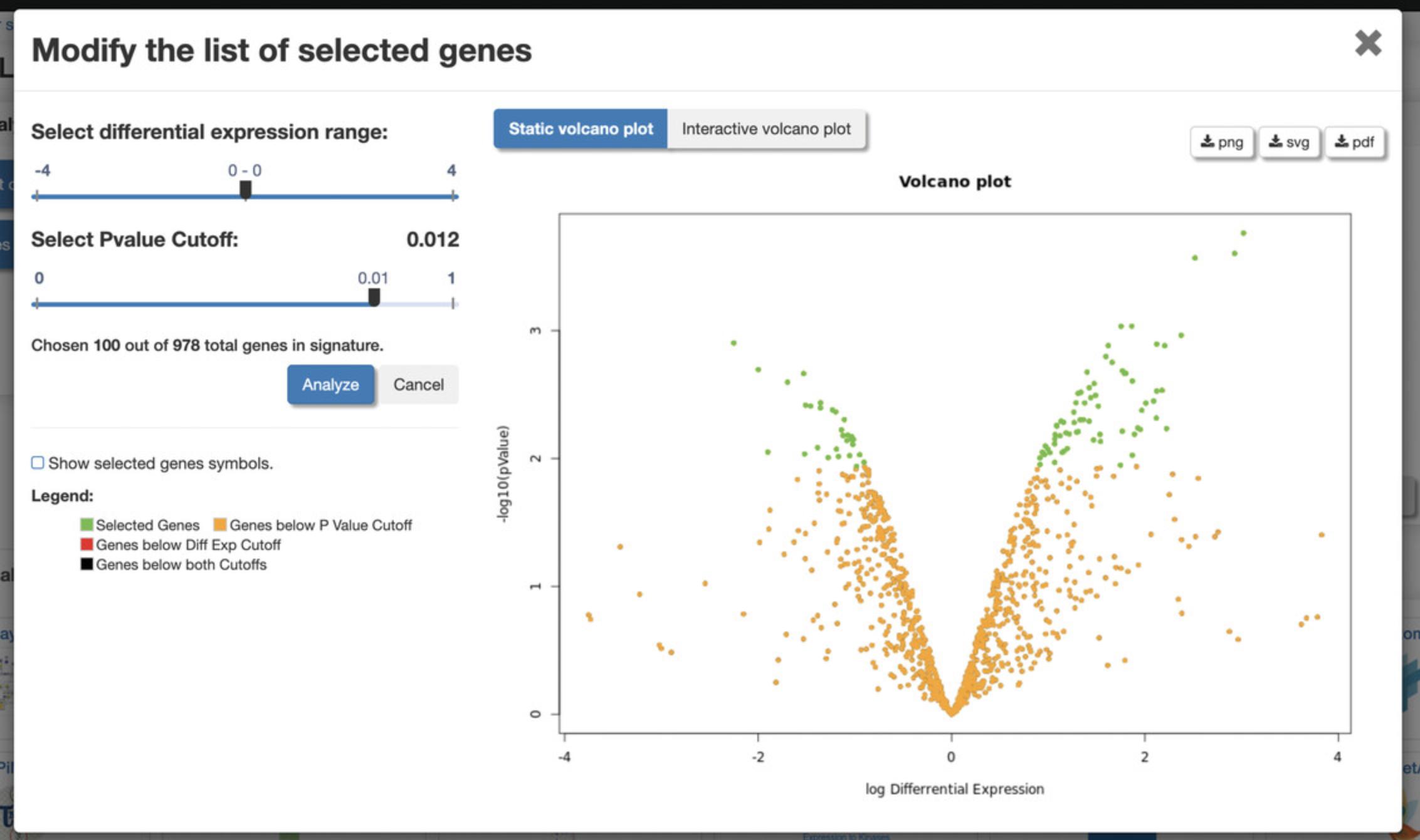
6.Click the “Modify the list of selected genes” button on the left to generate a volcano plot of differentially expressed genes (Fig. 115). The top 100 differentially expressed genes are selected by default. Use the sliders to change the differential expression range and p- value cutoff to change the number of top differentially expressed genes. Change between a static volcano plot and interactive volcano plot by clicking the “Static volcano plot” or “Interactive volcano plot” button. Click on any of the download buttons to download the volcano plot in the preferred file format.
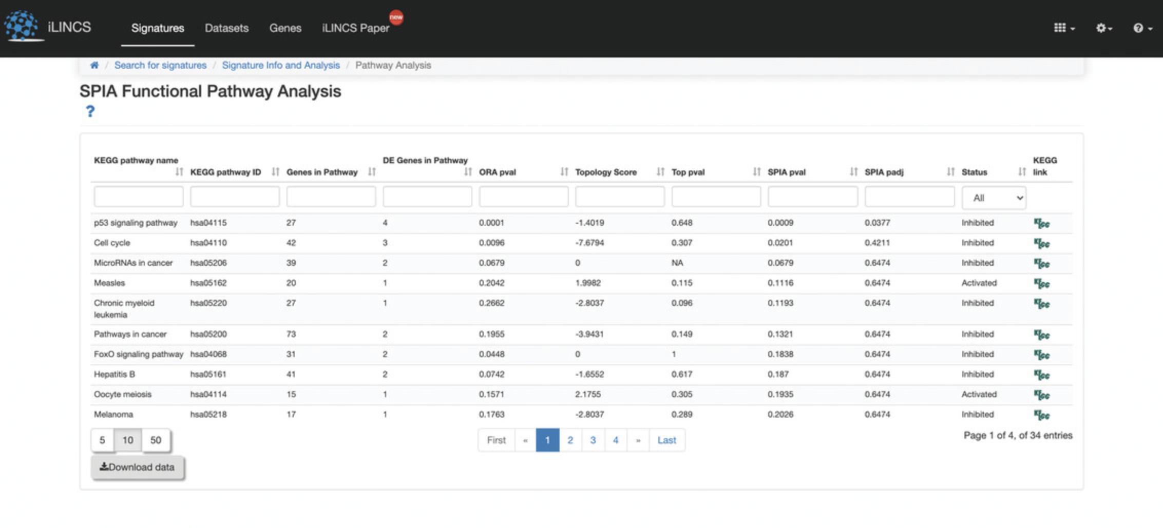
7.Several signature analysis tools are available for further exploration and visualization of the selected signature. Mouse over any of the signature analysis tools buttons to display a pop-up box with information, and click on any of the buttons to launch the analysis. As an example, click the “Pathway Analysis” button to be redirected to a new page with a SPIA Functional Pathway Analysis table of the top enriched KEGG pathways computed from the differentially expressed genes from the query signature (Fig. 116).
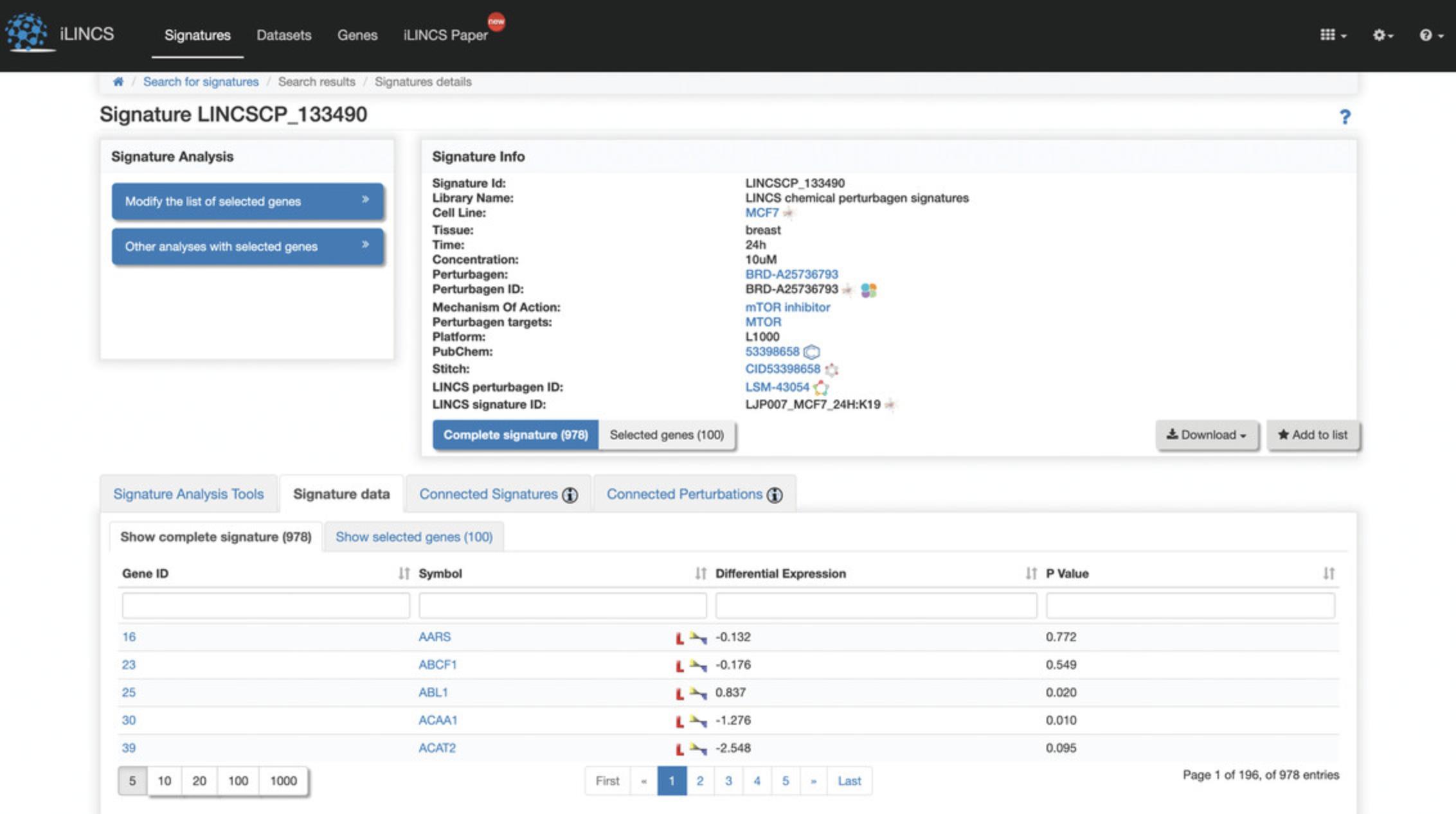
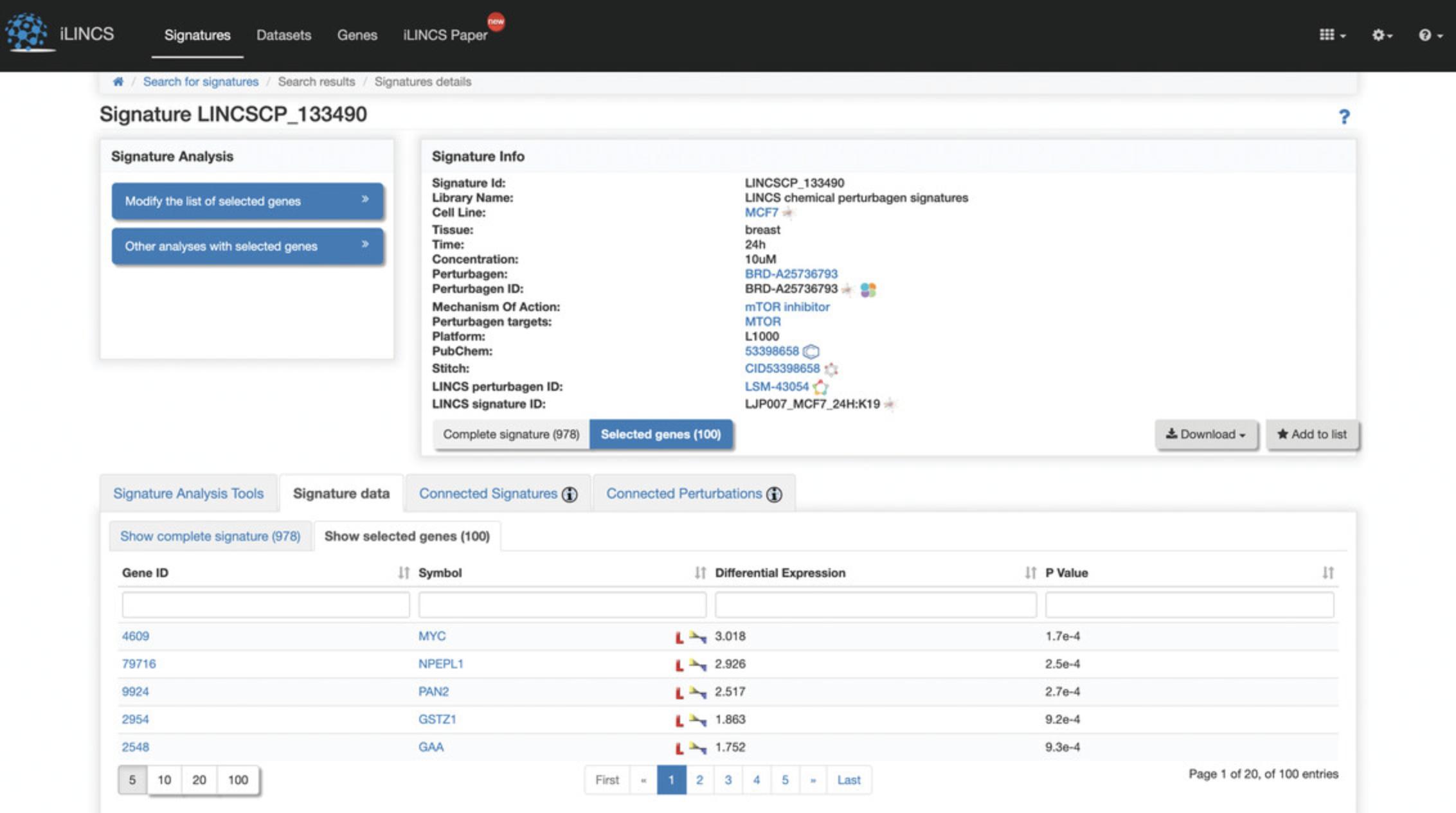
8.Click the “Signature data” tab at the bottom of the page to display a table of the genes included in the signature and their differential expression levels and p- values (Fig. 117). Click on “Show selected genes” within the tab to view the top 100 differentially expressed genes that are computed by default and their expression levels and p- values (Fig. 118). To change the selected genes, see step 6.
Connected Signatures
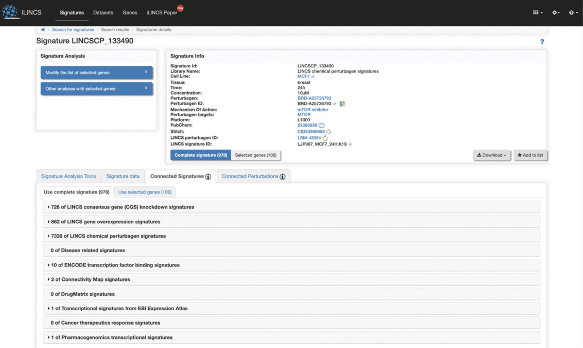
9.Click the “Connected Signatures” tab to view other pre-computed signatures connected to the selected signature based on Pearson correlation coefficient concordance (Fig. 119). As an example, expand the tab labeled “LINCS chemical perturbagen signatures” to display a table of chemical perturbagen signatures correlated to the selected signature. The table displays metadata for each signature, in addition to the concordance values, p- values, and number of overlapping genes (Fig. 120). Bar plots of top occurring perturbagens, targets, concentrations, cell lines, and time points across the signatures are displayed above the table.
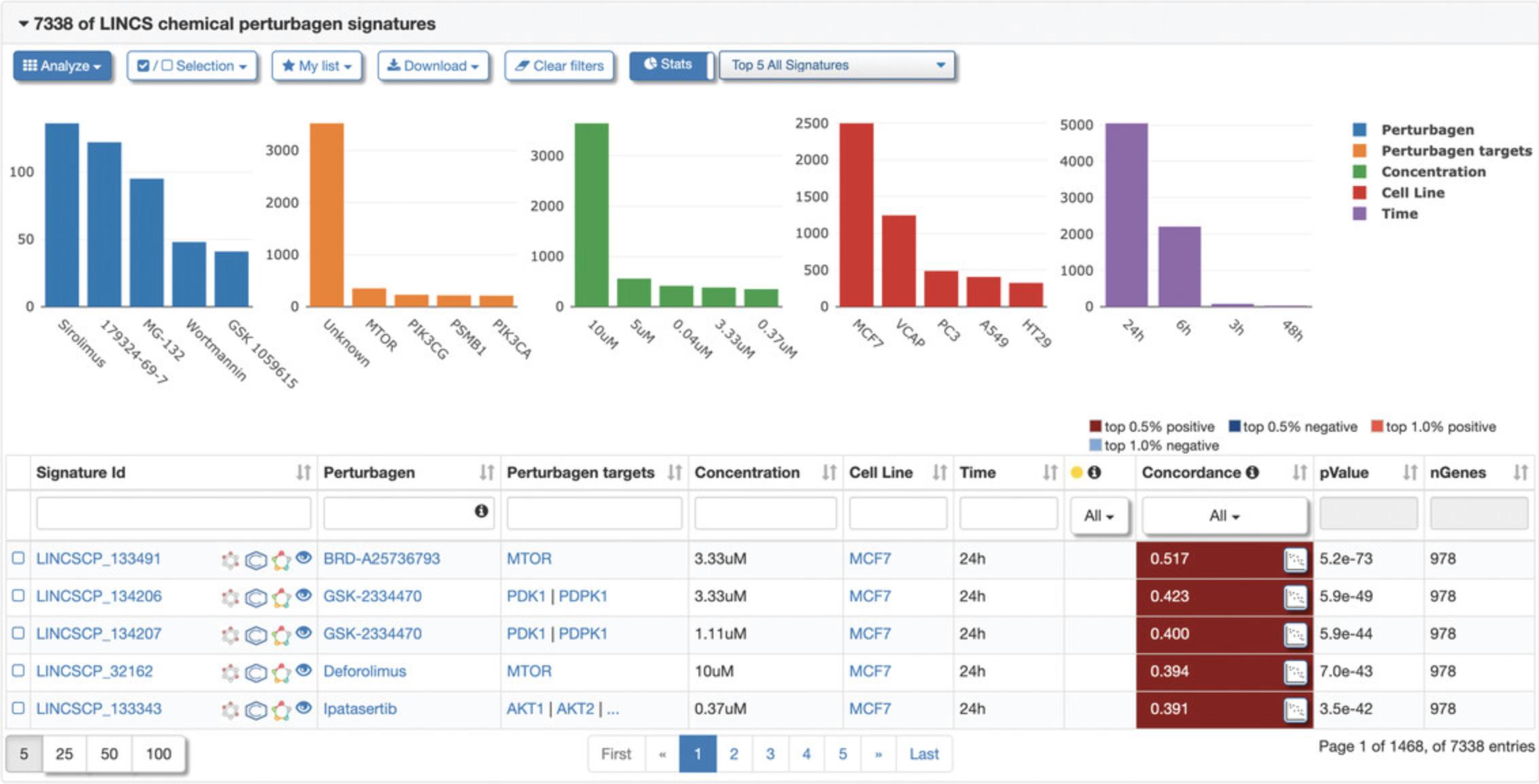
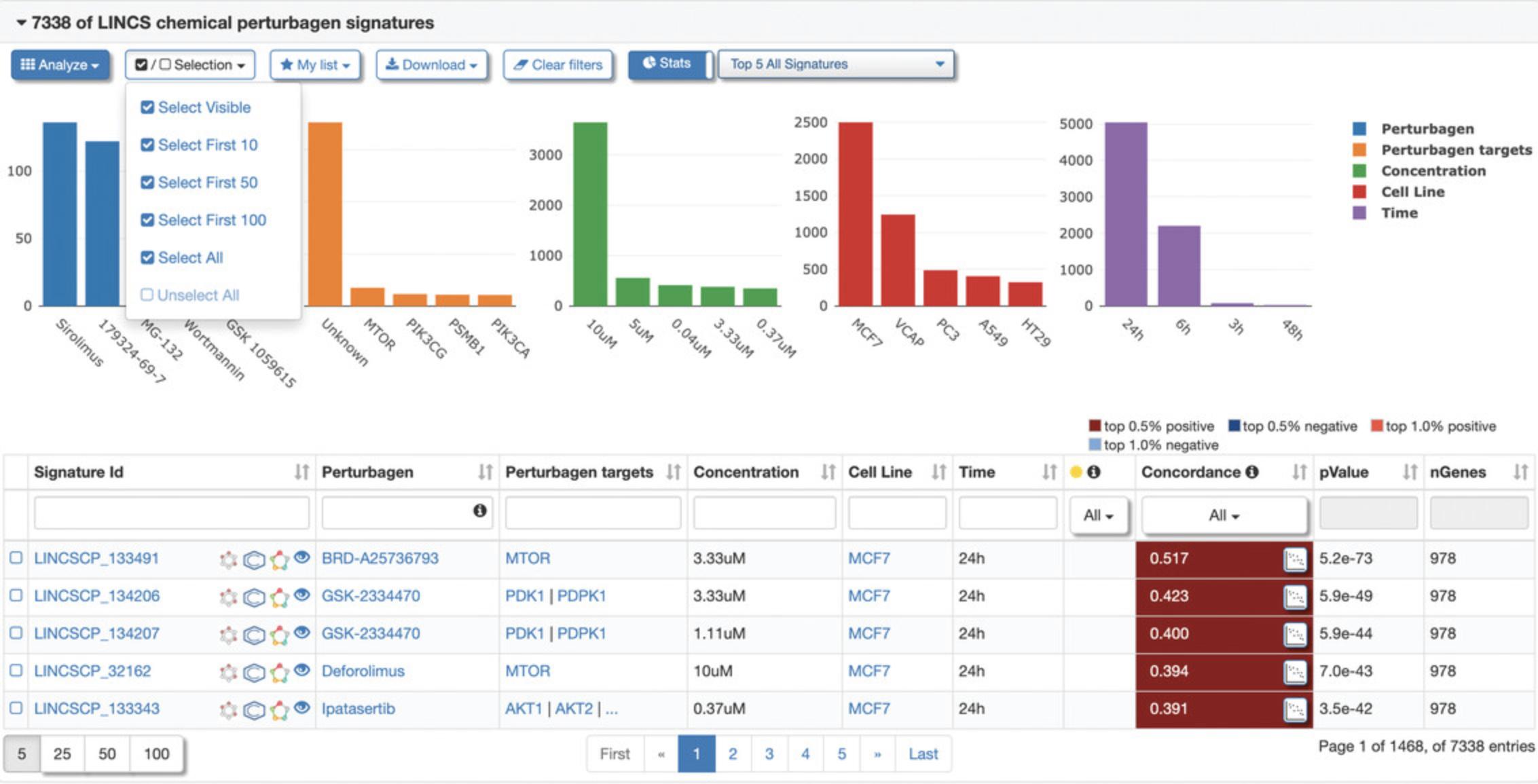
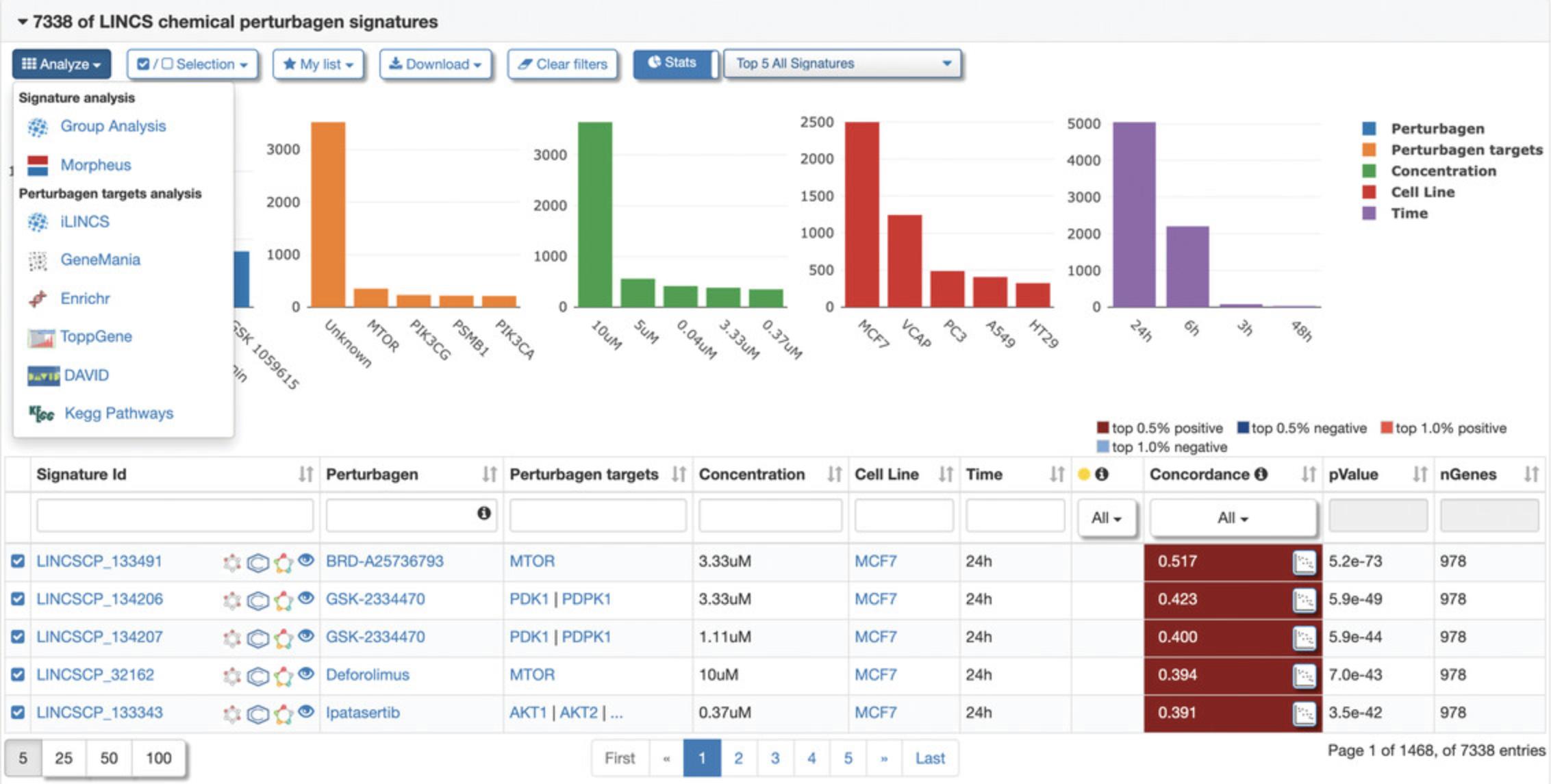
10.To select a group of signatures for analysis, click the “Selection” drop-down menu and click “Select First 100” to select the top 100 correlated chemical perturbagen signatures to the query signature, as indicated by a checkbox to the left of the Signature ID (Fig. 121). All other signatures after the first 100 will be unselected, as indicated by an unchecked box. Different signature groupings can be selected and deselected within the menu. Next, click the “Analyze” drop-down menu and select “Group Analysis” to perform a signature group analysis on the selected signatures (Fig. 122).
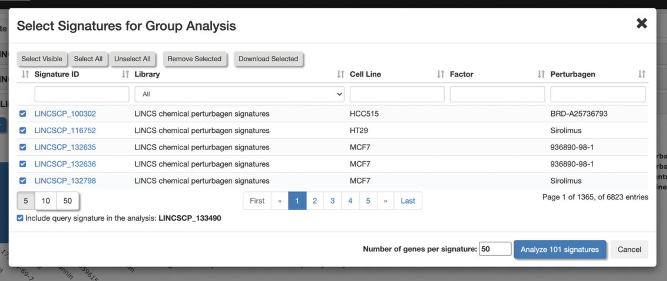
11.A pop-up menu will appear with a table of the selected signatures where signatures can once again be selected and deselected (Fig. 123). By default, 50 genes from each signature will be used in the analysis, but this field can be changed with the desired number of genes. Click “Analyze 100 signatures”.
12.A new page will be generated with a table of the selected signatures, which can be downloaded as signature data or a correlation matrix (Fig. 124). At the bottom of the page are analyses from various tools for clustering and visualizing the submitted signatures. As an example, click “Morpheus Signatures Heatmap”.
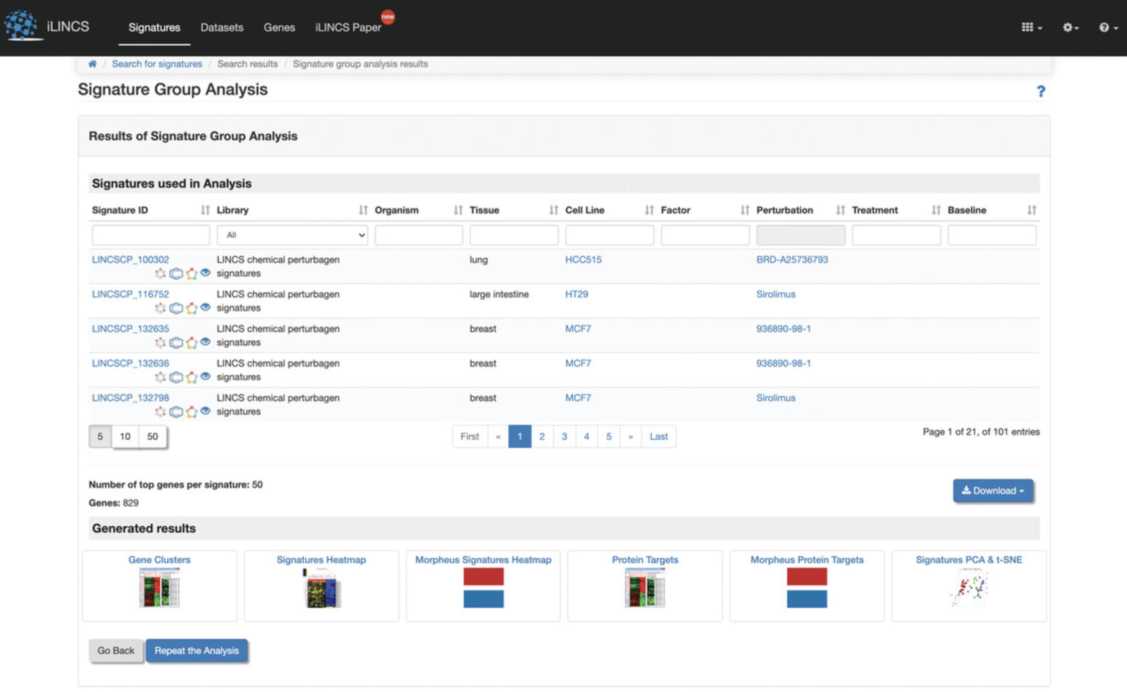
13.A new page will be generated with a heatmap of the submitted signatures clustered by the various metadata associated with each signature, like perturbagens, cell lines, etc. (Fig. 125).
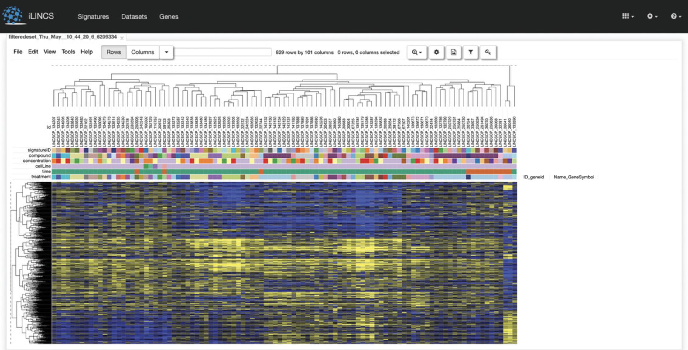
Connected Perturbations
14.Navigate back to the Signature Details page and click on the “Connected Perturbations” tab (Fig. 126). This tab includes aggregated tables of correlated gene knockdown and chemical perturbagen signatures.
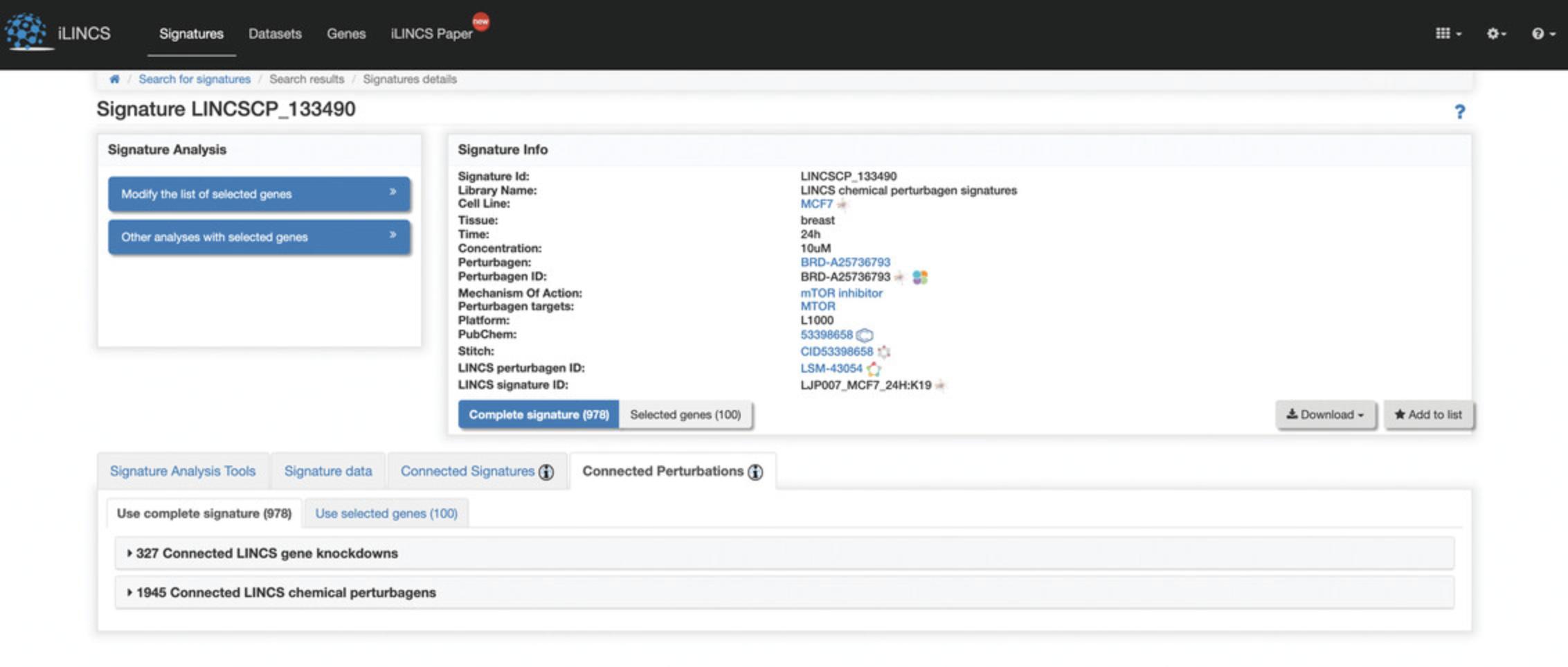
15.Expand the “LINCS gene knockdowns” tab to view the top correlated knockdown signatures with the query signature (Fig. 127). The table includes the target genes and pathways in addition to the various metrics that qualify the knockdown signatures as related to the query signature.
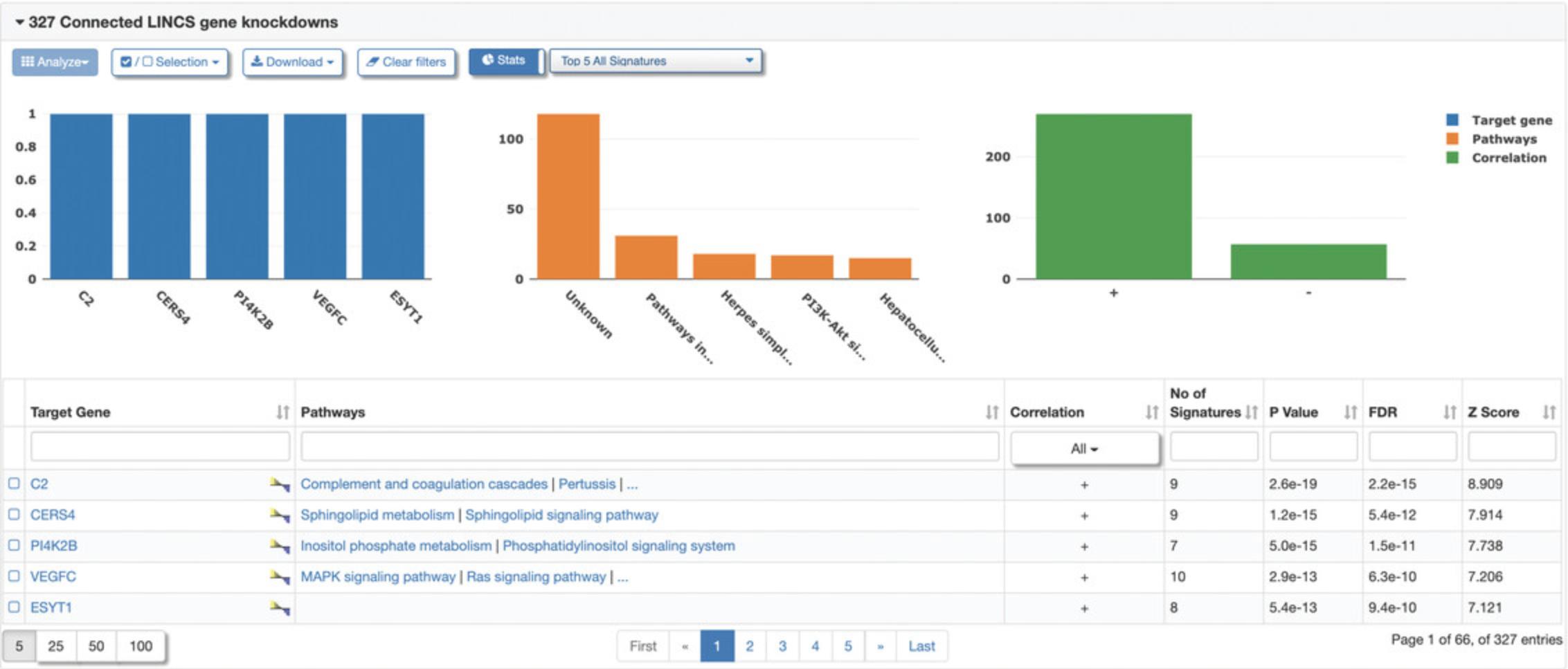
16.Expand the “LINCS chemical perturbagens” tab to view the top correlated perturbagen signatures with the query signature (Fig. 128). The table includes the perturbagen id, perturbagen name, and perturbagen targets in addition to the various metrics that qualified the perturbagen signatures as related to the query signature.
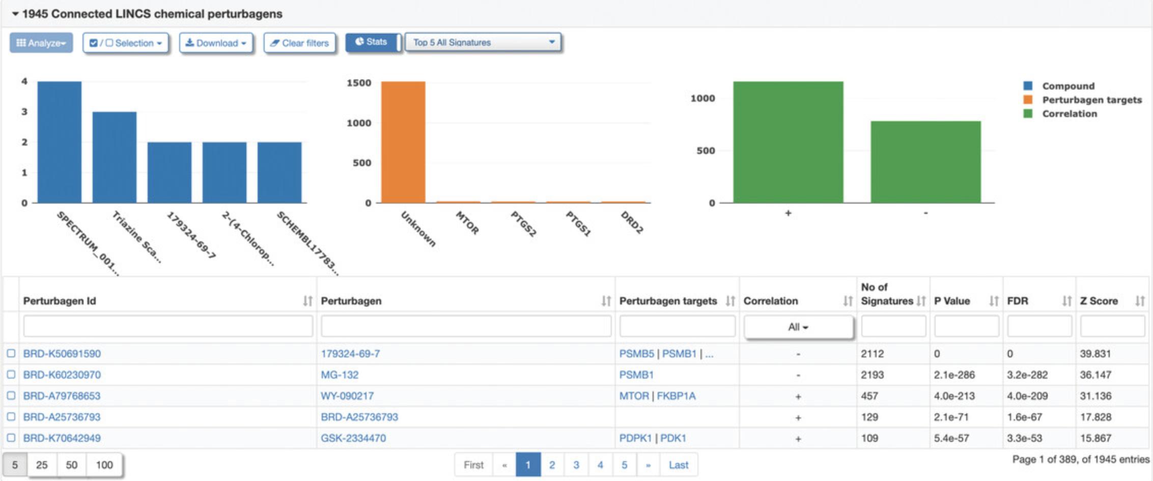
Creating and analyzing signatures
17.Switch to the datasets workflow by clicking on the “Datasets” button in the navigation bar at the top of the page. This page includes over 15,000 datasets of pre-processed signatures (Fig. 129). Select and deselect datasets of interest and use the drop-down menus on the right to narrow the search to terms of interest. For the demo, select only the “TCGA” dataset, select proteomics data from the “Data Type” drop-down menu, and type breast into the keyword search bar to narrow the search to datasets with proteomic data related to breast cancer (Fig. 130). To explore and analyze a dataset, click the “Analyze” button in the “TCGA_BRCA_RPPA_2019” dataset.
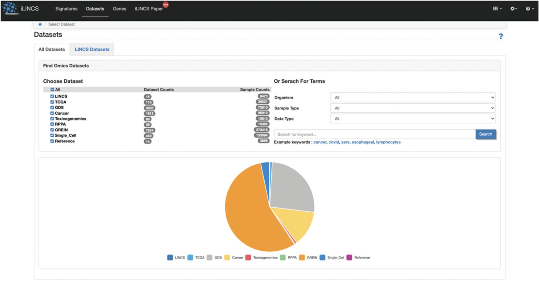
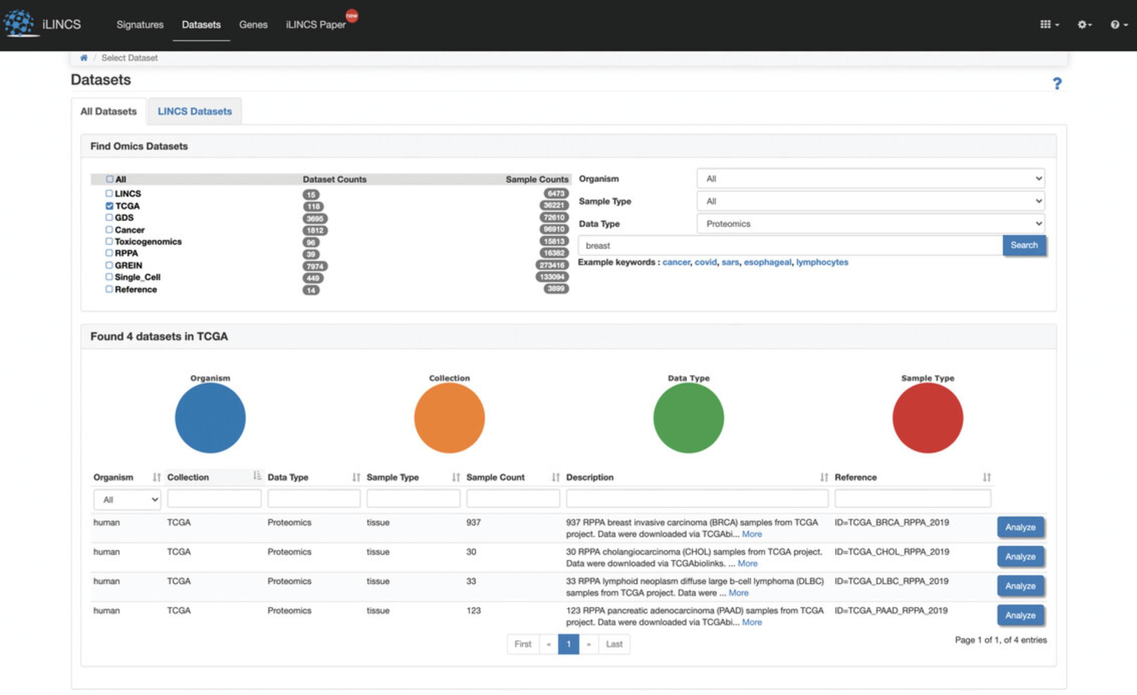
18.To create a signature, click the “Create a signature” button on the left (Fig. 131). On the left are drop-down menus of variables to separate the samples into two groups for comparison. For the grouping variable, select “PAM50_mRNA”. For the treatment group, select “HER-2 enriched” samples. For the baseline group, select “Luminal A” samples (Fig. 132). Once the grouping criteria are selected, click “Create signature” to generate the signature.
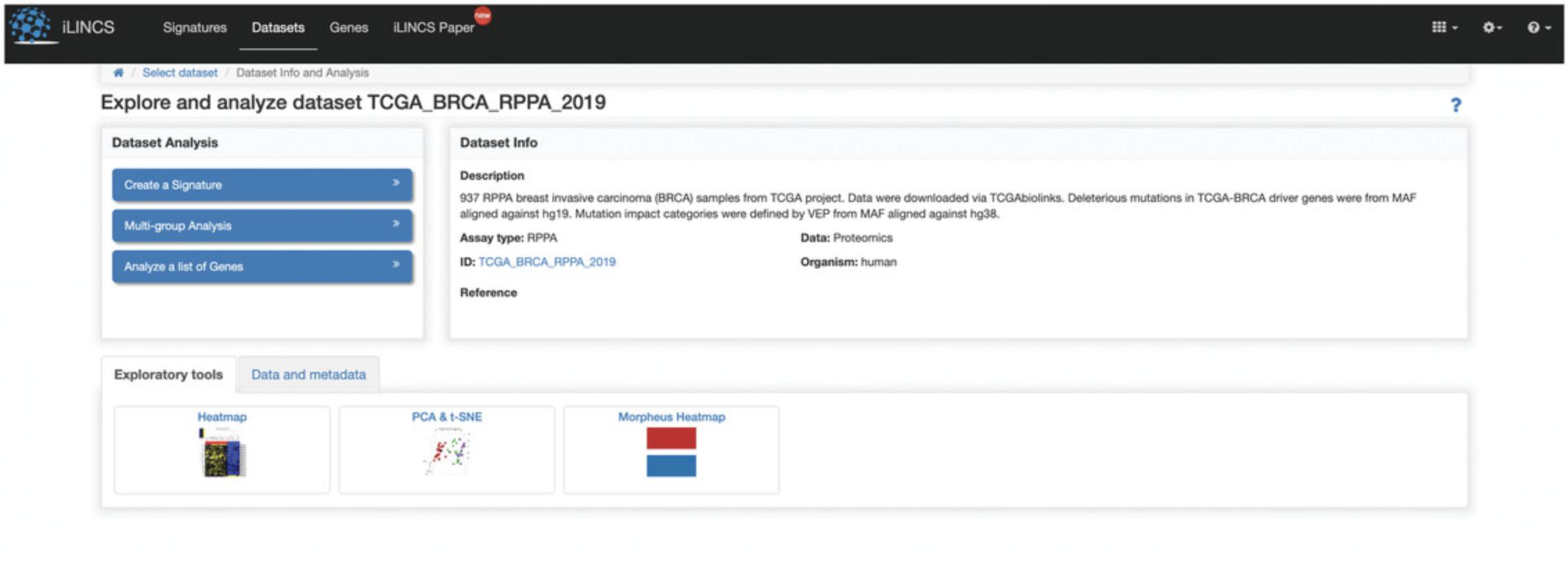

19.A signature details page will be created for the generated signature (Fig. 133). To further explore and analyze the signature follow steps 6-16.
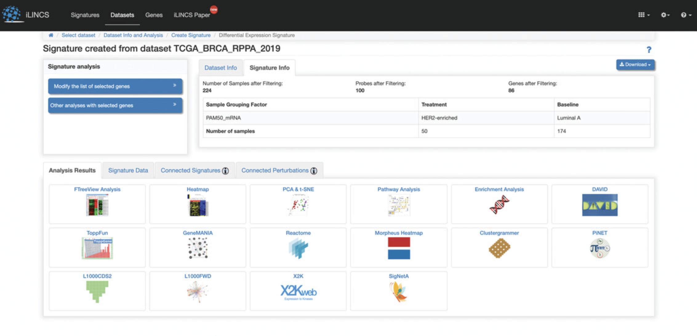
COMMENTARY
Background Information
The LINCS program consisted of six Data and Signature Generation Centers (DSGCs) and one Data Coordination and Integration Center (DCIC). Although funding for the LINCS program has ended and no new LINCS datasets are expected to be produced and published, the DCIC and each of the DSGCs continue to host existing data and develop new software tools. All the software tools mentioned in the protocols presented here will be available in the foreseeable future. A few new software tools and platforms, such as SigCom LINCS (Evangelista et al., 2022) and Appyters (Clarke et al., 2021), are still being actively developed (as of 2022), and the LINCS DCIC is committed to maintaining and upgrading these resources in the coming years.
In addition, the LINCS DCIC is participating in the Common Fund Data Ecosystem (CFDE) NIH Common Fund program. This effort aims to standardize metadata across NIH Common Fund data coordination centers (DCCs) (Charbonneau et al., 2022). For the CFDE efforts, most of the LINCS data and metadata have been archived on an Amazon Web Services S3 bucket using a STRIDES account. Persistent download links for these datasets can be found within LINCS metadata tables now available from the CFDE portal (https://app.nih-cfde.org/) and SigCom LINCS.
The LINCS Data Coordination and Integration Center (DCIC)
The LINCS DCIC focused on four main aspects: (1) constructing an integrated knowledge environment for accessing LINCS data; (2) conducting research on regulatory networks with LINCS data; (3) establishing community training and outreach opportunities centered on LINCS data; and (4) coordinating the activities of the consortium and involvement of LINCS in other efforts. Although the LINCS program period has ended, the LINCS DCIC continues to engage in outreach activities and provide access to LINCS digital resources.
The Drug Toxicity Signature Generation Center (DToxS) DSGC
The Drug Toxicity Signature (DToxS) DSGC generated cellular signatures related to adverse drug effects, with the goal of mitigating these effects via the coadministration of other drugs. Transcriptomics and proteomics data were collected from multiple cell lines that were treated with either single drugs or complementary drug combinations. This experimental data was then computationally analyzed to generate sets of signatures for each single drug or drug pair.
The Harvard Medical School (HMS) LINCS DSGC
The HMS LINCS DSGC aimed to understand the underlying mechanisms of drug sensitivity and dose-response relationships by studying cellular responses to small molecule perturbations, with a focus on kinase inhibitors, epigenome modifiers, and ligands. Data was collected via mRNA profiling, mass spectrometry proteomics, immunoassays, and cell imaging.
The LINCS Center for Transcriptomics DSGC
The LINCS Center for Transcriptomics generated a comprehensive collection of transcriptomic profiles, including the L1000 dataset, which expands upon the original Connectivity Map (CMAP; Lamb et al., 2006). The L1000 dataset covers over 50 cell types, to which nearly 82,000 perturbagens were applied at varying doses and timepoints (Subramanian et al., 2017). This DSGC has produced a staggering collection of over 3 million gene expression profiles to date.
The LINCS Proteomic Characterization Center for Signaling and Epigenetics (PCCSE) DSGC
The LINCS Proteomic Characterization Center for Signaling, and Epigenetics (PCCSE) collected data on changes in phosphorylation and protein expression in response to various perturbations. Data were measured using the P100 and Global Chromatin Profiling (GCP) assays. The PCCSE also collaborated with the LINCS Center for Transcriptomics to integrate L1000 transcriptomic data with PCCSE experiments.
The Microenvironment Perturbagen (MEP) LINCS DSGC
The Microenvironment Perturbagen (MEP) LINCS DSGC examined the effects of the microenvironment on cellular phenotypes and molecular networks. MEP LINCS data integrates quantitative fluorescence imaging-based assays with transcriptional and proteomics data to provide a comprehensive view of how microenvironment perturbagens affect regulatory networks.
The NeuroLINCS DSGC
The NeuroLINCS DSGC aimed to identify targets for the development of drugs against neurodegenerative diseases, focusing on amyotrophic lateral sclerosis (ALS) and spinal muscular atrophy (SMA). NeuroLINCS data consists of transcriptomics, proteomics, and imaging profiles of motor neurons (iMNs) derived from induced pluripotent stem cell (iPSC) technologies.
Critical Parameters
Workflow for the L1000 Assay
The workflow to measure gene expression with the L1000 assay involves ligation-mediated amplification (LMA) followed by fluorescently addressed microspheres to capture amplification products (Subramanian et al., 2017).
- In Step 1, mRNA is reverse transcribed into cDNA.
- In Steps 2 and 3, landmark gene–specific upstream and downstream probes are annealed to the cDNA, and then ligated. The upstream probe has a unique 24-mer barcoded sequence and a 50-biotin label.
- In Steps 4 to 6, the probes are amplified via polymerase chain reaction (PCR) using biotinylated primers, and are hybridized to polystyrene microspheres (beads) of distinct fluorescent colors, via their barcodes. Each bead recognizes two barcodes; many amplified molecules that feature either barcode can attach to a bead. To permit each bead to be analyzed for both color (indicating landmark transcript identity) and fluorescence intensity (indicating landmark abundance), streptavidin-phycoerythrin (SAPE) staining of biotin is performed. The beads are then sent to Luminex FlexMap 3D flow cytometry detectors to measure how many probes are hybridized. This produces the L1000 Level 1 data, which is the raw, unprocessed flow cytometry data from the Luminex scanners. L1000 experiments involve the use of 384-well plates, with approximately 18 control replicates per plate. Each batch includes 2-4 plates, representing ∼366 samples per batch.
L1000 Data Levels
The L1000 data is available at different levels of processing; each level of processing is associated with a Level number:
- Level 1: Raw, unprocessed flow cytometry data from Luminex scanners.
- Level 2: Gene expression values per 1000 genes after deconvolution from Luminex beads.
- Level 3: Gene expression profiles of both directly measured landmark transcripts and inferred genes, normalized using invariant set scaling followed by quantile normalization.
- Level 4: Signatures with differentially expressed genes computed by robust z- scores for each profile relative to the population control.
- Level 5: Processed signatures computed from replicate profiles using the moderated z- score (MODZ) method.
P100/GCP Data Levels
The P100 assay measures a reduced representation of the phosphoproteome consisting of 96 widely studied phosphopeptides. The P100 profiles of uncharacterized perturbations can be compared against profiles of drugs with known signaling pathways, and this way the signaling mechanisms of novel perturbagens can be inferred. The global chromatin profiling (GCP) assay measures global post-translational histone modifications in bulk chromatin. Using this platform, epigenetic signatures can be generated for small-molecule and genetic perturbations of epigenetic processes. The P100 and GCP assay data are available at different levels of processing, like the L1000 data:
- Level 0: Raw mass spectrometry data
- Level 1: Probe reads in the form of curated Skyline documents
- Level 2: Raw matrix data of extracted signal ratios of probes vs. internal standards (log2 transformed)
- Level 3: Processed and normalized matrix data derived from Level 2
- Level 4: Differential matrix data generated by subtracting each sample from Level 3 by the plate-wide median ratio of each analyte
Troubleshooting
Table 1 lists common problems that may arise with these protocols, along with their possible causes and solutions.
| Problem | Possible cause | Solution |
|---|---|---|
| Missing or inaccessible data on any LINCS data repository | The data is not available to non-registered users, or is unavailable for some other reason (e.g., unpublished data) | If creating an account is possible, do so and re-try downloading the data. Otherwise, contact site administrators or the relevant DSGC. |
| There is a bug in a LINCS tool | The tool and/or data used may require upgrading | Contact the DSGC responsible for the site. Some tools may be linked to GitHub repositories, in which case an issue may be created on the repository. |
| Deprecated LINCS data and tools | Because the LINCS program has ended, there may not be further updates or support for parts of LINCS data and software tools | It is still possible that existing LINCS datasets may be periodically updated based on new quality control and analysis procedures. Administrators at the DSGCs sites can provide information about whether updates should be expected. The LINCS DCIC is still actively developing and maintaining LINCS tools and databases, and most of these tools can be reliably accessed to analyze LINCS data. The LINCS DCIC provides support via online forms and e-mail. |
Acknowledgments
This work was partially supported by NIH grants OT2OD030160, U54HL127624 and OT3OD025459.
Author Contributions
Zhuorui Xie : writing original draft, developing tools, testing tools, producing figures, adding content, developing tutorials, reviewing and collating text, and editing; Eryk Kropiwnicki : writing original draft, testing tools, producing figures, adding content, developing tutorials, reviewing and collating text, and editing; Megan L. Wojciechowicz : developing tutorials, adding content, and editing; Kathleen M. Jagodnik : writing original draft, testing tools, producing figures, adding content, developing tutorials, reviewing and collating text, and editing; Ingrid Shu : developing tutorials, producing figures, adding content, and editing; Allison Bailey : developing tutorials, producing figures, adding content, and editing; Daniel J. B. Clarke : developing tools, adding content, and editing; Minji Jeon : developing tools, adding content, and editing; John Erol Evangelista : developing tools, adding content, and editing; Maxim Kuleshov : developing tools; Alexander Lachmann : developing tools; Abhijna A. Parigi : reviewing text; Jose M. Sanchez : reviewing text; Sherry L. Jenkins : project administration, supervision, reviewing and editing; Avi Ma'ayan : conceptualization, funding acquisition, project administration, supervision, writing original draft, reviewing and editing.
Conflict of Interest
The authors declare no conflict of interest.
Open Research
Data Availability Statement
Data sharing is not applicable to this article as no new data were created or analyzed in this study.
Literature Cited
- Barretina, J., Caponigro, G., Stransky, N., Venkatesan, K., Margolin, A. A., Kim, S., … Garraway, L. A. (2012). The Cancer Cell Line Encyclopedia enables predictive modelling of anticancer drug sensitivity. Nature , 483(7391), 603–607. doi: 10.1038/nature11003
- Charbonneau, A. L., Brady, A., Czajkowski, K., Aluvathingal, J., Canchi, S., Carter, R., … White, O. (2022). Making Common Fund data more findable: Catalyzing a Data Ecosystem. bioRxiv , doi: 10.1101/2021.11.05.467504
- Clark, N. A., Hafner, M., Kouril, M., Williams, E. H., Muhlich, J. L., Pilarczyk, M., … Medvedovic, M. (2017). GRcalculator: An online tool for calculating and mining dose–response data. BMC Cancer , 17(1), 698. doi: 10.1186/s12885-017-3689-3
- Clark, N. R., Hu, K. S., Feldmann, A. S., Kou, Y., Chen, E. Y., Duan, Q., & Ma'ayan, A. (2014). The characteristic direction: A geometrical approach to identify differentially expressed genes. BMC Bioinformatics , 15(1), 79. doi: 10.1186/1471-2105-15-79
- Clarke, D. J. B., Jeon, M., Stein, D. J., Moiseyev, N., Kropiwnicki, E., Dai, C., … Ma'ayan, A. (2021). Appyters: Turning Jupyter Notebooks into data-driven web apps. Patterns , 2(3), 100213–100213. doi: 10.1016/j.patter.2021.100213
- Clarke, D. J. B., Kuleshov, M. V., Schilder, B. M., Torre, D., Duffy, M. E., Keenan, A. B., … Ma'ayan, A. (2018). eXpression2Kinases (X2K) Web: Linking expression signatures to upstream cell signaling networks. Nucleic Acids Research , 46(W1), W171–W179. doi: 10.1093/nar/gky458
- Duan, Q., Reid, S. P., Clark, N. R., Wang, Z., Fernandez, N. F., Rouillard, A. D., … Ma'ayan, A. (2016). L1000CDS2: LINCS L1000 characteristic direction signatures search engine. NPJ Systems Biology and Applications , 2(1), 16015. doi: 10.1038/npjsba.2016.15
- Edgar, R., Domrachev, M., & Lash, A. E. (2002). Gene Expression Omnibus: NCBI gene expression and hybridization array data repository. Nucleic Acids Research , 30(1), 207–210. doi: 10.1093/nar/30.1.207
- Enache, O. M., Lahr, D. L., Natoli, T. E., Litichevskiy, L., Wadden, D., Flynn, C., … Subramanian, A. (2019). The GCTx format and cmap{Py, R, M, J} packages: Resources for optimized storage and integrated traversal of annotated dense matrices. Bioinformatics , 35(8), 1427–1429. doi: 10.1093/bioinformatics/bty784
- Evangelista, J. E., Clarke, D. J. B., Xie, Z., Lachmann, A., Jeon, M., Chen, K., … Ma'ayan, A. (2022). SigCom LINCS: Data and metadata search engine for a million gene expression signatures. Nucleic Acids Research , gkac328. doi: 10.1093/nar/gkac328
- Fabian, M. A., Biggs, W. H. 3rd, Treiber, D. K., Atteridge, C. E., Azimioara, M. D., Benedetti, M. G., … Lockhart, D. J. (2005). A small molecule-kinase interaction map for clinical kinase inhibitors. Nature Biotechnology , 23(3), 329–336. doi: 10.1038/nbt1068
- Fabregat, A., Jupe, S., Matthews, L., Sidiropoulos, K., Gillespie, M., Garapati, P., … D'Eustachio, P. (2018). The Reactome Pathway Knowledgebase. Nucleic Acids Research , 46(D1), D649–d655. doi: 10.1093/nar/gkx1132
- Fernandez, N. F., Gundersen, G. W., Rahman, A., Grimes, M. L., Rikova, K., Hornbeck, P., & Ma'ayan, A. (2017). Clustergrammer, a web-based heatmap visualization and analysis tool for high-dimensional biological data. Scientific Data , 4(1), 170151. doi: 10.1038/sdata.2017.151
- GTEx Consortium. (2020). The GTEx Consortium atlas of genetic regulatory effects across human tissues. Science , 369(6509), 1318–1330. doi: 10.1126/science.aaz1776
- Kanehisa, M., & Goto, S. (2000). KEGG: Kyoto encyclopedia of genes and genomes. Nucleic Acids Research , 28(1), 27–30. doi: 10.1093/nar/28.1.27
- Koleti, A., Terryn, R., Stathias, V., Chung, C., Cooper, D. J., Turner, J. P., … Schürer, S. C. (2018). Data Portal for the Library of Integrated Network-based Cellular Signatures (LINCS) program: Integrated access to diverse large-scale cellular perturbation response data. Nucleic Acids Research , 46(D1), D558–D566. doi: 10.1093/nar/gkx1063
- Kuleshov, M. V., Jones, M. R., Rouillard, A. D., Fernandez, N. F., Duan, Q., Wang, Z., … Ma'ayan, A. (2016). Enrichr: A comprehensive gene set enrichment analysis web server 2016 update. Nucleic Acids Research , 44(W1), W90–97. doi: 10.1093/nar/gkw377
- Kutmon, M., Riutta, A., Nunes, N., Hanspers, K., Willighagen, E. L., Bohler, A., … Pico, A. R. (2016). WikiPathways: Capturing the full diversity of pathway knowledge. Nucleic Acids Research , 44(D1), D488–494. doi: 10.1093/nar/gkv1024
- Lamb, J., Crawford, E. D., Peck, D., Modell, J. W., Blat, I. C., Wrobel, M. J., … Golub, T. R. (2006). The Connectivity Map: Using gene-expression signatures to connect small molecules, genes, and disease. Science , 313(5795), 1929–1935. doi: 10.1126/science.1132939
- Litichevskiy, L., Peckner, R., Abelin, J. G., Asiedu, J. K., Creech, A. L., Davis, J. F., … Jaffe, J. D. (2018). A library of phosphoproteomic and chromatin signatures for characterizing cellular responses to drug perturbations. Cell System , 6(4), 424–443.e427. doi: 10.1016/j.cels.2018.03.012
- Niepel, M., Hafner, M., Duan, Q., Wang, Z., Paull, E. O., Chung, M., … Sorger, P. K. (2017). Common and cell-type specific responses to anti-cancer drugs revealed by high throughput transcript profiling. Nature Communications , 8(1), 1186. doi: 10.1038/s41467-017-01383-w
- Niepel, M., Hafner, M., Mills, C. E., Subramanian, K., Williams, E. H., Chung, M., … Sorger, P. K. (2019). A multi-center study on the reproducibility of drug-response assays in mammalian cell lines. Cell System , 9(1), 35–48.e35. doi: 10.1016/j.cels.2019.06.005
- Pilarczyk, M., Kouril, M., Shamsaei, B., Vasiliauskas, J., Niu, W., Mahi, N., … Medvedovic, M. (2020). Connecting omics signatures of diseases, drugs, and mechanisms of actions with iLINCS. bioRxiv , 826271. doi: 10.1101/826271
- Rouillard, A. D., Gundersen, G. W., Fernandez, N. F., Wang, Z., Monteiro, C. D., McDermott, M. G., & Ma'ayan, A. (2016). The harmonizome: A collection of processed datasets gathered to serve and mine knowledge about genes and proteins. Database , 2016, baw100. doi: 10.1093/database/baw100
- Sharma, V., Eckels, J., Schilling, B., Ludwig, C., Jaffe, J. D., MacCoss, M. J., & MacLean, B. (2018). Panorama Public: A Public Repository for Quantitative Data Sets Processed in Skyline. Molecular and Cell Proteomics , 17(6), 1239–1244. doi: 10.1074/mcp.RA117.000543
- Stathias, V., Turner, J., Koleti, A., Vidovic, D., Cooper, D., Fazel-Najafabadi, M., … Schürer, S. C. (2019). LINCS Data Portal 2.0: Next generation access point for perturbation-response signatures. Nucleic Acids Research , 48(D1), D431–D439. doi: 10.1093/nar/gkz1023
- Stathias, V., Turner, J., Koleti, A., Vidovic, D., Cooper, D., Fazel-Najafabadi, M., … Schürer, S. C. (2020). LINCS Data Portal 2.0: Next generation access point for perturbation-response signatures. Nucleic Acids Research , 48(D1), D431–D439. doi: 10.1093/nar/gkz1023
- Subramanian, A., Narayan, R., Corsello, S. M., Peck, D. D., Natoli, T. E., Lu, X., … Golub, T. R. (2017). A Next Generation Connectivity Map: L1000 Platform and the First 1,000,000 Profiles. Cell , 171(6), 1437–1452.e1417. doi: 10.1016/j.cell.2017.10.049
- Consortium, The Gene Ontology. (2019). The Gene Ontology Resource: 20 years and still GOing strong. Nucleic Acids Research , 47(D1), D330–D338. doi: 10.1093/nar/gky1055
- Torre, D., Lachmann, A., & Ma'ayan, A. (2018). BioJupies: Automated generation of interactive notebooks for RNA-Seq data analysis in the cloud. Cell System , 7(5), 556–561.e553. doi: 10.1016/j.cels.2018.10.007
- Wang, Z., Lachmann, A., Keenan, A. B., & Ma'ayan, A. (2018). L1000FWD: Fireworks visualization of drug-induced transcriptomic signatures. Bioinformatics , 34(12), 2150–2152. doi: 10.1093/bioinformatics/bty060
- Wang, Z., Monteiro, C. D., Jagodnik, K. M., Fernandez, N. F., Gundersen, G. W., Rouillard, A. D., … Ma'ayan, A. (2016). Extraction and analysis of signatures from the Gene Expression Omnibus by the crowd. Nature Communications , 7, 12846–12846. doi: 10.1038/ncomms12846
- Wilkinson, M. D., Dumontier, M., Aalbersberg, I. J., Appleton, G., Axton, M., Baak, A., … Mons, B. (2016). The FAIR Guiding Principles for scientific data management and stewardship. Scientific Data , 3(1), 160018. doi: 10.1038/sdata.2016.18
Internet Resources
NIH LINCS program website __
* <https://lincsproject.org/LINCS/>
The homepage for the LINCS Program. The overarching goals of the program are described here, as well as each of the DSGCs and the DCIC. Links to tools, publications, and data can also be found here.
Phase 1 L1000 data __
* <https://www.ncbi.nlm.nih.gov/geo/query/acc.cgi?acc=GSE92742>
The LINCS Phase 1 L1000 dataset, released in 2016, contains the first ∼1.3 million gene expression profiles generated by the L1000 platform. This dataset is available on GEO via accession GSE92742, under the “Supplementary Files” section, and includes downloadable data for each of the five levels of the L1000 data; Level 5 signatures are computed using the moderated z-score. Additionally, a Readme file and 10 metadata files are provided.
LINCS 2020 L1000 data __
* <https://clue.io/releases/data-dashboard>
The LINCS 2020 L1000 data, provides over 3 million gene expression profiles. Additional perturbagens and cell lines beyond those from Phase 1 have been added, including hematopoietic cell lines and non-cancer-related cell lines.
L1000 Profiles of GTEx data __
* <https://www.ncbi.nlm.nih.gov/geo/query/acc.cgi?acc=GSE92743>
As part of the process of validating and improving the L1000 assay, GTEx samples were profiled using both L1000 and RNA-seq assays. Both sets of data are available from GEO series GSE92743.
Notebooks providing L1000 data access __
* <https://github.com/cmap/lincs-workshop-2020>
The LINCS Center for Transcriptomics has created notebooks to provide various forms of access and interaction with the L1000 data. A cmapBQ tutorial notebook is provided, as is a cmapBQ Toolkit Demo notebook. Additionally, for gene expression analysis, the Compound Dose Response notebook and the Gene Modulation notebook are available. For cell fitness analysis, notebooks are provided for Exploration of Prism Cell Viability Data and for Cell Growth Rate and Impact on Viability Profiles. Documentation is provided for each notebook.
DToxS Center website __
* <https://martip03.u.hpc.mssm.edu/>
Information on the DToxS DSGC is provided at this site. All data, metadata, and signatures for DToxS data are also available with creation of an account. Metadata are available for cells, drugs, and assays. Twenty-eight standard operating procedures (SOPs) are also available in the categories of Cell SOPs, Assay SOPs, and Computational SOPs.
HMS LINCS database __
* <https://lincs.hms.harvard.edu/db/>
Data and metadata from HMS LINCS transcriptomics studies are hosted here, including data for KINOMEscan and KiNativ. Metadata are provided for all datasets, as well as cells, kinases, and small molecules.
The Drug-Pathway Browser __
* <https://lincs.hms.harvard.edu/explore/pathway/>
This tool provides an interactive network map of signal transduction pathways. Users can identify compounds that target a particular kinase or are associated with a phenotype of interest, or identify compounds having similar or synergistic effects via involvement in the same signal transduction cascade. Compound, protein, and cell lines are hyperlinked to their corresponding entries in the HMS LINCS Database.
The HMS LINCS Breast Cancer Browser __
* <http://www.cancerbrowser.org/>
Both published and unpublished datasets related to the biology of breast cancer and associated drug response are hosted here. Datasets include the Basal Receptor (RTK) Profile data, the Basal Total Protein Mass Spectrometry data, the Basal Phosphoprotein Mass Spectrometry dataset, the Growth Factor-Induced pAKT/pERK Response data, and the Drug Dose-Response Growth Rate Profiling dataset. The website also provides a Cell Line view for exploring each breast cancer cell line in depth, as well as a Drugs view containing information on drug development, function, and targets.
CLUE.io __
* <https://clue.io/>
The CLUE platform provides both a data portal for the L1000 data and a set of tools for working with the L1000 data. This platform requires the creation of a free account to log in and access its resources. Included are the CLUE Repurposing App, which permits users to explore drugs and tool compounds to identify drug repurposing opportunities to advance disease treatment; the CLUE Touchstone App, which provides interactive plots and permits users to explore connectivity among drug, loss-of-function, and gain-of-function signatures via interactive plots; the CLUE Morpheus App, which provides heat map analyses of data from the LINCS Center for Transcriptomics data and also allows for uploading and analyzing user data; and the CLUE Cell App, which permits the exploration of various cell lines and their annotations.
L1000FWD __
* <https://maayanlab.cloud/L1000FWD/>
The L1000FWD platform (Wang et al., 2018) provides an interactive scatter plot visualization of over 17,000 drug-induced transcriptomics signatures. The app also allows for viewing signatures by cell line or small molecule, as well as querying user-submitted signatures to find the top drugs to mimic or reverse a signature.
L1000CDS2 __
* <https://maayanlab.cloud/L1000CDS2/#/index>
The L1000CDS2 platform (Duan et al., 2016) takes user-submitted signatures or gene sets and returns consensus L1000 characteristic direction signatures that mimic or reverse the input signature.
iLINCS __
* <http://www.ilincs.org/ilincs/>
iLINCS (Pilarczyk et al., 2020) is a cloud-based platform that allows access to LINCS data as well as various workflows for processing and analyzing transcriptomics and proteomics data.
LINCS Data Portal v1 __
* <http://lincsportal.ccs.miami.edu/dcic-portal/>
The LINCS Data Portal v1 (Koleti et al., 2018) provides a data repository for earlier LINCS data releases prior to the 2020 data release. 422 LINCS datasets are accessible and available for download on the website, and can be queried by metadata, such as the small molecules, cells, genes, proteins, and antibodies studied. Assay and DSGC information are also provided for each dataset.
LINCS Data Portal v2 __
* <http://lincsportal.ccs.miami.edu/signatures/home>
The LINCS Data Portal v2 (Stathias et al., 2020) provides an updated user interface and enhanced metadata annotation to the LINCS Data Portal v1. Querying by signatures via the iLINCS platform (Pilarczyk et al., 2020), and by chemical structures are supported in addition to metadata queries.
SigCom LINCS __
* <https://maayanlab.cloud/sigcom-lincs>
SigCom LINCS is the latest LINCS data portal. It contains the most recent release of LINCS data. In addition to metadata and signature search functionalities, detailed and interactive visualizations of the LINCS data and metadata are provided. SigCom LINCS also contains signatures from other sources, gene pages, FAIR assessments of LINCS data, a downloads page, and OpenAPI programmatic access. SigCom LINCS search functionality includes single gene search, and the automatic conversion of any search term to gene sets and signatures.
Citing Literature
Number of times cited according to CrossRef: 2
- Zhuorui Xie, Clara Chen, Avi Ma’ayan, Dex-Benchmark: datasets and code to evaluate algorithms for transcriptomics data analysis, PeerJ, 10.7717/peerj.16351, 11 , (e16351), (2023).
- Yasha Hasija, Bioinformatics workflow management systems, All About Bioinformatics, 10.1016/B978-0-443-15250-4.00006-X, (247-265), (2023).

