FLASH-seq UMI protocol

Prepare the following lysis mix:

A	B	C	D
Reagent	Reaction concentration	Volume (µl)	384-well plate
Triton-X100 (10% v/v)	0.2%	0.020	8.448
dNTP mix (25 mM each)	6 mM	0.240	101.376
STRT-P1-T31 oligo (100 µM)	1.8 µM	0.018	7.603
RNAse inhibitor (40 U/µl)	1.2 U/µl	0.030	12.672
DTT (100 mM)	1.2 mM	0.012	5.069
dCTP (100 mM)	9 mM	0.090	38.016
Betaine (5 M)	1 M	0.200	84.480
Nuclease-free water	-	0.390	164.736
Total volume (µl)		1.000	422.400

Add 1µL lysis buffer to each well of a 384-well plate.

Seal the plate with a PCR seal and quickly spin it down to collect the lysis buffer to the bottom.

Proceed immediately to the next step or store the plate at -20°C long-term. Plates that are going to be used on the same day can be stored in the fridge or kept on wet ice.

Sort single cells into 384-well plates containing 1µL lysis buffer.

Seal the plate with an aluminium seal. If processing multiple plates at once, keep each of them on dry ice until ready to transfer them all at -80°C for long-term storage. Plates containing single cells should ideally be processed within 6 months.

Remove the plates from the -80°C freezer and check that the aluminium seal is still intact. If damaged or not sticking to the plate anymore, wait a few minutes for the plate to partially thaw, remove the damaged foil and replace it with a new one.

Place the plate in a thermocycler with a heated lid and incubate for 0h 3m 0s at 72°C, followed by a 4°C hold step.

Spin down any condensation droplets that may have formed during the incubation and return the plate to a cool rack. Proceed quickly to the next step. If not ready with the RT-PCR mix, keep the plate on the cool rack at all times.

While the plate is in the thermocycler, prepare the following RT-PCR mix:

A	B	C	D
Reagent	Reaction concentration	Volume (µl)	384-well plate
DTT (0.1 M)	4.8 mM	0.238	100.531
MgCl2 (1 M)	9.2 mM	0.046	19.430
Betaine (5 M)	800 mM	0.800	337.920
RNAse inhibitor (40 U/µl)	0.8 U/µl	0.096	40.550
SuperScript IV (200 U/µl)	2.00 U/µl	0.050	21.120
KAPA HiFi HotStart Ready Mix (2 x)	1 x	2.500	1056.000
TSO-UMI (100 µM)	1.84 µM	0.092	38.861
Tn5_ISPCR- F (100 µM)	0.5 µM	0.025	10.560
DI-PCR-P1A-R (100 µM)	0.1 µM	0.005	2.112
Nuclease-free water	-	0.148	62.515
Total volume (µl)		4.000	1689.600

Add 4µL RT-PCR mix into each well of the 384-well plate.

Seal the plate with a PCR seal, gently vortex and spin down to collect the liquid to the bottom.

Place it in a thermocycler with heated lid and start the following RT-PCR program:

A	B	C	D	E
Step		Temperature	Time	Cycles
RT		50ºC	60 min	1 x
PCR	initial denaturation	98ºC	3 min	1 x
	denaturation	98ºC	20 sec	20-24 x*
	annealing	65ºC	20 sec
	elongation	72ºC	6 min
		15ºC	Hold

*Adjust the number according to the cell type used. We recommend 20-21 cycles for HEK 293T cells and 23-24 cycles for hPBMC. The addition of UMI and the lack of semi-suppressive PCR decreases reaction yield. As a rule of thumb, we typically start our testing with the same number of PCR cycles as in the SMART-seq2 protocol.

For the Magnetic beads working solution preparation users are referred to the standard FLASH-seq protocol (section 5).

Remove the Sera-Mag SpeedBeads™ working solution (or AMPure XP beads or SPRI beads when using a commercial solution) from the 4°C storage and equilibrate it at room temperature for 0h 15m 0s.

Add a 0.6 x ratio of Sera-Mag SpeedBeads™ working solution to each well (i.e., 9 μl beads for each 15 μl cDNA). Mix thoroughly by pipetting or vortexing.

Incubate the plate off the magnetic stand for 0h 5m 0s at 4Room temperature.

Place the plate on the magnetic stand and leave it for 0h 5m 0s or until the solution appears clear.

Remove the supernatant without disturbing the beads.

Performing an ethanol wash is not required but possible. We do not recommend it when working in 384-well plates and with liquid handling robots to avoid cDNA losses.

Remove the plate from the magnetic stand, add 15µLnuclease-free water and mix well by pipetting or vortexing to resuspend the beads. Do not let the bead pellet to dry completely, as that lowers the final cDNA yield!

Incubate 0h 2m 0s off the magnetic stand.

Place the plate back on the magnetic stand and incubate for 0h 2m 0s or until the solution appears clear.

Remove 14µL of the supernatant and transfer it to a new plate.

Check the cDNA quality on Agilent Bioanalyzer High Sensitivity DNA chip. Follow the instructions as described in the user manual. A good sample is characterized by a low proportion of fragments <400 bp, absence of residual primers (ca. 100 bp) and an average cDNA size of 1.8–2.2 Kb.

Example of amplified cDNA from a single HEK 293T cell (21 cycles).

For the cDNA quantification users are referred to the standard FLASH-seq protocol (section 8).

Prepare a normalization plate by adding 1µL of purified cDNA and nuclease-free water to a final concentration of 100pg/μl.

Prepare the tagmentation mix as described below:

A	B
Reagent	Volume (µl)
ATM (Amplification Tagment Mix)	0.1 to 0.2*
TD (Tagmentation DNA buffer)	1
Total volume (µl)	1.1 to 1.2

*If the cDNA quantification is accurate, then 0.1-0.2 μl should give sequencing-ready libraries in the range of 700-1000 bp. Fragments of >1000 bp are not expected to efficiently bind to the NextSeq or NovaSeq flow cells and should therefore be avoided.

Dispense 1.2µL tagmentation mix in a new 384-well plate.

Add 1µL normalized cDNA (100pg/μl) to each well containing the Tagmentation Mix.

Seal the plate, vortex, spin down, and carry out the tagmentation reaction: 55°C for 0h 8m 0s, 4°C hold. Upon completion proceed immediately to the next step.

Add 0.5µL 0.2% SDS to each well. Seal the plate, vortex, spin down and incubate 5 min at room temperature. Do not put the plate back on ice.

Add 1µL N7xx + S5xx Index Adaptors (5micromolar (µM) each).

Add 1.5µL Nextera PCR Mix (NPM) to each well:

Seal the plate, vortex, spin down, and place it in a thermocycler and carry out the Enrichment PCR Reaction:

A	B	C	D	E
Step		Temperature	Time	Cycles
Gap filling		72ºC	3 min	1 x
enrichment PCR	initial denaturation	95ºC	30 sec	1 x
	denaturation	95ºC	10 sec	14 x
	annealing	55ºC	30 sec
	elongation	72ºC	30 sec
		15ºC	hold

Take an aliquot from each sample for the final library cleanup (the rest can be stored long-term at -20°C) and transfer it to a 1.5-ml Eppendorf tube.

Remove the Sera-Mag SpeedBeads™ working solution (alternatively: AMPure XP beads or SPRI beads) from the 4°C storage and equilibrate it at 4Room temperature for 0h 15m 0s.

Add Sera-Mag SpeedBeads™ working solution to a final ratio of 0.8 x and mix well to homogenization.

Incubate the tube off the magnetic stand for 0h 5m 0s at room temperature.

Place the tube on the magnetic stand and leave it for 0h 5m 0s or until the solution appears clear.

Remove the supernatant without disturbing the beads.

Recommended: wash the pellet with 1mLof 80% v/v ethanol. Incubate 0h 0m 30s without removing the tube from the magnetic stand.

Remove any trace of ethanol and let the bead pellet dry for 0h 2m 0s or until small cracks appear. Do not cap the tube or remove it from the magnetic stand during this time.

Remove the tube from the magnetic stand, add 50µL nuclease-free water and mix well by pipetting or vortexing to resuspend the beads.

Incubate 0h 2m 0s off the magnetic stand.

Place the tube back on the magnetic stand and incubate for 0h 2m 0s or until the solution appears clear.

Remove 49µL of the supernatant and transfer it to a new 1.5-ml LoBind tube. Store the cDNA in a -20°C freezer long-term or until ready for sequencing.

Check the final library size on the Agilent Bioanalyzer. Follow the instructions as described in the High Sensitivity DNA chip user manual.

Use Qubit fluorometer or a similar fluorimetric assay to quantify the library.

Use the average size indicated on the Bioanalyzer and the concentration reported after Qubit measurement to determine the exact molarity required for sequencing.

Example of a sequencing-ready library from a pool of HEK 293T cells. Average size around 800 bp.

The purified library can be sequenced on any Illumina sequencer. Follow the specifications reported for each instrument. Depending on your application, single-end or paired-end reads (recommended) can be used. The read 1 length should not be <75 bp and preferably ≥100 bp. We regularly sequence FS-UMI libraries on a NextSeq550 using 100-8-8-50 read mode but preliminary data indicate that 90-8-8-60 or 80-8-8-70 read modes might lead to better results.

These instructions briefly describe the data processing of the sequencing results. The final pipeline will likely have to be adapted to the question at hand. The following lines assume that all the programs and their dependencies are installed on your machine and that the data are paired-end reads. Some values, such as the number of threads and RAM usage may have to be adapted to your machine settings.

The analysis of internal / UMI reads from full-length single-cell RNA-sequencing protocol is still in its infancy. This pipeline is therefore likely to evolve in the future. Please refer to the work of Hagemann-Jensen et al which first described this approach in SMART-seq3 for additional information.

We present this analysis for internal and UMI reads separately.

Prerequisites: bcl2fastq, umi_tools, STAR, samtools, featurecounts, bbmap (optional), IGV (optional)

Sample demultiplexing

Sequencing results will be delivered as demultiplexed FASTQ or raw bcl2 files. To convert bcl2 files to FASTQ, bcl2fastq program (Illumina) can be used.

# 0. Variables
BASECALL_DIR="/path/to/flowcell/Data/Intensities/BaseCalls/"
OUTPUT_DIR="/path/to/output_folder/"
SAMPLESHEET="/path/to/Demultiplexing_SampleSheet.csv"

# 1. Bcl2fastq
ulimit -n 10000
cd /path/to/flowcell/
bcl2fastq --input-dir $BASECALL_DIR --output-dir $OUTPUT_DIR --sample-sheet $SAMPLESHEET --create-fastq-for-index-reads --no-lane-splitting

When sequencing on a Nextseq500 instrument, the sample sheet should contain the following information in a csv file:

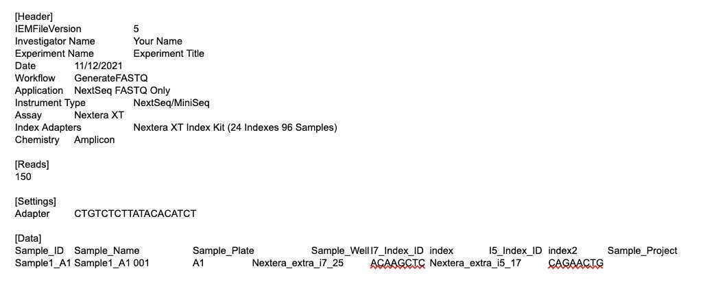
Illumina Experiment Manager can be used to assist you in creating the sample sheet.

We recommend exploring the barcode combinations left in the undetermined reads looking to confirm that all the cells have been properly demultiplexed.

zcat Undetermined_S0_I1_001.fastq.gz | awk -F' 1:N:0:' 'NR%4==1{print $2}' | sort | uniq -c > left_index.txt
sort -k1,1 left_index.txt
```as well as the read distribution between samples:

for file in ./out/R1 do zcat $file | wc -l done

Count Matrix - UMI

mkdir FEATURECOUNTS
 
# 1. Assign UMI reads to features
featureCounts -T 1 -p -t exon -g gene_name -s 1 --fracOverlap 0.25 -a "$GTF" -R BAM -o FEATURECOUNTS/"$ID"_Aligned.txt STAR/"$ID"_UMI_Aligned.sortedByCoord.filtered.bam
	
# 2. Sort and Index Reads
samtools sort  -@ 10 FEATURECOUNTS/"$ID"_UMI_Aligned.sortedByCoord.filtered.bam.featureCounts.bam -o FEATURECOUNTS/"$ID"_UMI_Aligned.sortedByCoord.filtered.bam.featureCounts.sorted.bam
samtools index FEATURECOUNTS/"$ID"_UMI_Aligned.sortedByCoord.filtered.bam.featureCounts.sorted.bam

# 3. Deduplicate and Count UMI Reads
umi_tools count --per-gene --paired --gene-tag=XT --chimeric-pairs=discard --unpaired-reads=discard --assigned-status-tag=XS -I FEATURECOUNTS/"$ID"_UMI_Aligned.sortedByCoord.filtered.bam.featureCounts.sorted.bam -S FEATURECOUNTS/"$ID".umi.counts.tsv.gz

Count Matrix - Internal

mkdir FEATURECOUNTS
featureCounts -T 1 -p -t exon -g gene_name --fracOverlap 0.25 -a "$GTF" -o FEATURECOUNTS/"$ID"_INTERNAL_featureCounts.txt STAR/"$ID"_INTERNAL_Aligned.sortedByCoord.filtered.bam

Post-Processing

The post-processing steps will vary depending on the question at hand. The online book “Orchestrating Single-Cell Analysis with Bioconductor” (https://bioconductor.org/books/release/OSCA/) is a gold mine of information that can be used to help you design your own pipeline. Alternatively, Seurat (R, https://satijalab.org/seurat/) or scanpy (python, https://scanpy.readthedocs.io/en/stable/) provide tools compatible with FLASH-Seq data.

Index the genome

The reference genome needs to be indexed prior to any mapping. The FASTA and GTF references can be obtained from ENSEMBL, Gencode, UCSC, ...

The optimal sjdbOverhang value should be set to the max(mate length) - 1.

# 0. Variables
OUTPUTREF="/path/to/STAR_indexed_genome/"
FASTA="GRCh38.primary_assembly.genome.fa"
GTF="gencode.v34.primary_assembly.annotation.gtf"

# 1. Genome indexing
# sjdbOverhang should be adapted based on the read length (read_length - 1)
mkdir $OUTPUTREF

STAR --runThreadN 15 --runMode genomeGenerate --genomeDir $OUTPUTREF --genomeFastaFiles $FASTA --sjdbGTFfile $GTF --sjdbOverhang 99

UMI extraction

The UMI sequence is located in read 1 (R1). However, a smaller proportion of UMI sequences can also be observed in read 2 (R2) due to tagmentation events occurring upstream of the UMI sequence, in the 5’ adapter. The following lines allow you to retrieve UMI sequences from both reads.

Assuming that the spacer sequence is “CTAAC”:

# 1. Extract UMI in read 1
umi_tools extract --bc-pattern="^(?P<discard_1>AAGCAGTGGTATCAACGCAGAGT|AGCAGTGGTATCAACGCAGAGT|GCAGTGGTATCAACGCAGAGT|CAGTGGTATCAACGCAGAGT|AGTGGTATCAACGCAGAGT|GTGGTATCAACGCAGAGT|TGGTATCAACGCAGAGT|GGTATCAACGCAGAGT|GTATCAACGCAGAGT|ATCAACGCAGAGT|CAACGCAGAGT|AACGCAGAGT|ACGCAGAGT|GCAGAGT|CAGAGT|AGAGT|GAGT|AGT|GT)(?P<umi_1>.{8})(?P<discard_2>CTAACGG)(?P<discard_3>G{0,4})" --stdin=sample.R1.fastq.gz --stdout=umi.UMIinR1.R1.fq --read2-in=sample.R2.fastq.gz --read2-out=umi.UMIinR1.R2.fq --extract-method=regex



# 2. Extract UMI in read 2
umi_tools extract --bc-pattern="^(?P<discard_1>GAGT|AGT|GT)(?P<umi_1>.{8})(?P<discard_2>CTAACGG)(?P<discard_3>G{0,4})" --stdin=sample.R2.fastq.gz --stdout=umi.UMIinR2.R2.fq --read2-in=sample.R1.fastq.gz --read2-out=umi.UMIinR2.R1.fq --extract-method=regex

# 3. In very rare cases (<0.0001%) can get the UMI in both R1 and R2. Find read IDs with a UMI in both R1 and R2
cat umi.UMIinR1.R1.fq | uniq | awk 'NR%4==1{print}' | sed 's/\@//g' > names.R1umi.txt
cat umi.UMIinR2.R1.fq | uniq | awk 'NR%4==1{print}' | sed 's/\@//g' > names.R2umi.txt
cat names.R1umi.txt | sed 's/_........ .*$//g' > names.R1umi.cleaned
cat names.R2umi.txt | sed 's/_........ .*$//g' > names.R2umi.cleaned
comm -12 <(sort names.R1umi.cleaned) <(sort names.R2umi.cleaned) > R1R2.toFilterOut

echo "===> Number of R1-R2 with both a UMI: $(wc -l R1R2.toFilterOut) <==="
echo "===> Number of R1 UMI before cleanup: $(wc -l names.R1umi.txt) <==="
echo "===> Number of R2 UMI before cleanup: $(wc -l names.R2umi.txt) <==="

# 4. Filter out double UMI reads from UMI reads
grep -f R1R2.toFilterOut names.R1umi.txt > R1.toFilterOut
grep -f R1R2.toFilterOut names.R2umi.txt > R2.toFilterOut
$BBMAP_filter in=umi.UMIinR1.R1.fq in2=umi.UMIinR1.R2.fq out=umi.UMIinR1.R1.tmp out2=umi.UMIinR1.R2.tmp names=R1.toFilterOut include=f overwrite=t
$BBMAP_filter in=umi.UMIinR2.R1.fq in2=umi.UMIinR2.R2.fq out=umi.UMIinR2.R1.tmp out2=umi.UMIinR2.R2.tmp names=R2.toFilterOut include=f overwrite=t

mv umi.UMIinR1.R1.tmp umi.UMIinR1.R1.fq
mv umi.UMIinR2.R1.tmp umi.UMIinR2.R1.fq
mv umi.UMIinR1.R2.tmp umi.UMIinR1.R2.fq
mv umi.UMIinR2.R2.tmp umi.UMIinR2.R2.fq

echo "===> Number of R1 UMI after cleanup: $(grep -c \@ umi.UMIinR1.R1.fq) <==="
echo "===> Number of R2 UMI after cleanup: $(grep -c \@ umi.UMIinR2.R1.fq) <==="

Separate internal reads from UMI reads

# 1. Get Internal reads by excluding the UMI reads 
cat umi.UMIinR1.R1.fq | uniq | awk 'NR%4==1{print}' | sed 's/\@//g' | sed 's/_........//g' > names.R1umi.txt
cat umi.UMIinR2.R1.fq | uniq | awk 'NR%4==1{print}' | sed 's/\@//g' | sed 's/_........//g' > names.R2umi.txt
sed -i 's/_........//g' R1.toFilterOut
sed -i 's/_........//g' R2.toFilterOut
cat names.R1umi.txt names.R2umi.txt R1.toFilterOut R2.toFilterOut > names.umi.txt

$BBMAP_filter in=sample.R1.fastq.gz in2=sample.R2.fastq.gz out=internal.R1.fq out2=internal.R2.fq names=names.umi.txt include=f overwrite=t

echo "===> Number of Internal Reads after cleanup: $(grep -c \@ internal.R1.fq) <==="

Reconcile UMI reads with reference

UMI reads in read 1 are stranded (=same orientation as the reference). However, due to their sequencing, UMI reads originating from the read 2 are in opposite directions compared to the reference.

To reconcile both read type orientations, read 2 of “UMI in read 2” reads are to be considered as read 1. Similarly, read 1 from “UMI in read 2” are to be considered as read 2.

# 1. Combine
cat umi.UMIinR1.R1.fq umi.UMIinR2.R2.fq > umi.R1.fq
cat umi.UMIinR1.R2.fq umi.UMIinR2.R1.fq > umi.R2.fq

# 2. Final Clean-up
rm R1.toFilterOut R2.toFilterOut toFilterOut.txt
rm names.* umi.UMIinR*.R*.fq
```These orientation differences are the reason why we cannot simply look simultaneously for UMI in both R1 and R2 using umi_tools.

FASTQ Trimming (optional)

If you observe sequencing primer left-overs after extracting the UMI sequence, the FASTQ files can be trimmed using BBDUK or Trimmomatic.

# 1. Trim Reads
bbduk.sh -Xmx48g in1=FASTQ/umi.R1.fq in2=FASTQ/umi.R2.fq out1=FASTQ/umi.R1.2.fq out2=FASTQ/umi.R2.2.fq t=32 ktrim=l ref=adapters.fa k=23 mink=7 hdist=1 hdist2=0 minlength=29 tbo
bbduk.sh -Xmx48g in1=FASTQ/umi.R1.2.fq in2=FASTQ/umi.R2.2.fq out1=FASTQ/umi.R1.trim.fq out2=FASTQ/umi.R2.trim.fq t=32 ktrim=r ref=adapters.fa k=23 mink=7 hdist=1 hdist2=0 minlength=29 tbo

bbduk.sh -Xmx48g in1=FASTQ/internal.R1.fq in2=FASTQ/internal.R2.fq out1=FASTQ/internal.R1.2.fq out2=FASTQ/internal.R2.2.fq t=32 ktrim=l ref=adapters.fa k=23 mink=7 hdist=1 hdist2=0 minlength=29 tbo
bbduk.sh -Xmx48g in1=FASTQ/internal.R1.2.fq in2=FASTQ/internal.R2.2.fq out1=FASTQ/internal.R1.trim.fq out2=FASTQ/internal.R2.trim.fq t=32 ktrim=r ref=adapters.fa k=23 mink=7 hdist=1 hdist2=0 minlength=29 tbo

# 2. Rename
mv FASTQ/umi.R1.trim.fq FASTQ/umi.R1.fq
mv FASTQ/umi.R2.trim.fq FASTQ/umi.R2.fq
mv FASTQ/internal.R1.trim.fq FASTQ/internal.R1.fq
mv FASTQ/internal.R2.trim.fq FASTQ/internal.R2.fq

# 3. Clean-up
rm FASTQ/internal.R1.2.fq FASTQ/internal.R2.fq FASTQ/umi.R1.2.fq FASTQ/umi.R2.2.fq
```In the following line we treat UMI and internal reads separately. Depending on your needs, they can be used together as well.

Mapping UMI reads

The FASTQ file can then be mapped onto the reference genome. Example for one sample, use a loop or parallelise this task to process all the cells:

# 0. Variables
GENOME="/path/to/STAR_indexed_genome/"
FASTQ_R1="/path/to/umi.R1.fq”
FASTQ_R2="/path/to/umi.R2.fq"
ID=”sample_id”

# 1. Mapping
STAR --runThreadN 10 --limitBAMsortRAM 20000000000 --genomeLoad LoadAndKeep --genomeDir $GENOME --readFilesIn "$FASTQ_R1" "$FASTQ_R2" --readFilesCommand cat --limitSjdbInsertNsj 2000000 --seedSearchStartLmax 30 --outFilterIntronMotifs RemoveNoncanonicalUnannotated --outSAMtype BAM SortedByCoordinate --outFileNamePrefix STAR/"$ID"_UMI_


# 2. SAM to sorted BAM
# -F 260 filters out unmapped and secondary alignments
samtools view -@ 5 -Sb -F 260 "$ID"_UMI_Aligned.sortedByCoord.out.bam > "$ID"_UMI_Aligned.sortedByCoord.filtered.bam
samtools index "$ID"_UMI_Aligned.sortedByCoord.filtered.bam

Mapping Internal reads

# 0. Variables
GENOME="/path/to/STAR_indexed_genome/"
FASTQ_R1="/path/to/internal.R1.fq”
FASTQ_R2="/path/to/internal.R2.fq"
ID=”sample_id”

# 1. Mapping
mkdir STAR
STAR --runThreadN 10 --limitBAMsortRAM 20000000000 --genomeLoad LoadAndKeep --genomeDir $GENOME --readFilesIn "$FASTQ_R1" "$FASTQ_R2" --readFilesCommand cat --limitSjdbInsertNsj 2000000 --outFilterIntronMotifs RemoveNoncanonicalUnannotated --outSAMtype BAM SortedByCoordinate --outFileNamePrefix STAR/"$ID"_INTERNAL_

# 2. SAM to sorted BAM
# -F 260 filters out unmapped and secondary alignments
samtools view -@ 5 -Sb -F 260 "$ID"_INTERNAL_Aligned.sortedByCoord.out.bam > "$ID"_INTERNAL_Aligned.sortedByCoord.filtered.bam
samtools index "$ID"_INTERNAL_Aligned.sortedByCoord.filtered.bam

Data Visualization (optional)

Once the reads have been mapped we highly recommend using the Integrated Genome Viewer (IGV) to visualize the mapping results and ensure that the results make sense. As a quick check-up visualize a few housekeeping genes (i.e., ACTB, GAPDH, …) and cell specific markers to look for reads mapping to exon, intron, exon-intron junctions. UMI reads should mainly map to the 5’ of the gene in concordant orientation.

Look for abnormalities such as read piles falling in intergenic or centromeric regions.

No single-cell RNA sequencing protocol is perfect and non-specific priming, genomic DNA contaminations, … can happen but should represent rare events.

Recurrent soft-clipping could also indicate the presence of sequencing adaptor left-overs that could affect the mapping rate.