A metabolic modeling platform for the computation of microbial ecosystems in time and space (COMETS)
Ilija Dukovski, Djordje Bajić, Jeremy M. Chacón, Michael Quintin, Jean C. C. Vila, Snorre Sulheim, Alan R. Pacheco, David B. Bernstein, William J. Riehl, Kirill S. Korolev, Alvaro Sanchez, William R. Harcombe, Daniel Segrè


Extended
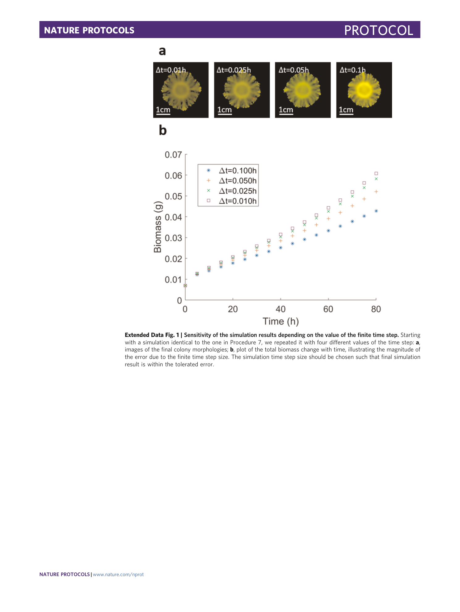
Extended Data Fig. 1 Sensitivity of the simulation results depending on the value of the finite time step.
Starting with a simulation identical to the one in Procedure 7, we repeated it with four different values of the time step: a , images of the final colony morphologies; b , plot of the total biomass change with time, illustrating the magnitude of the error due to the finite time step size. The simulation time step size should be chosen such that final simulation result is within the tolerated error.
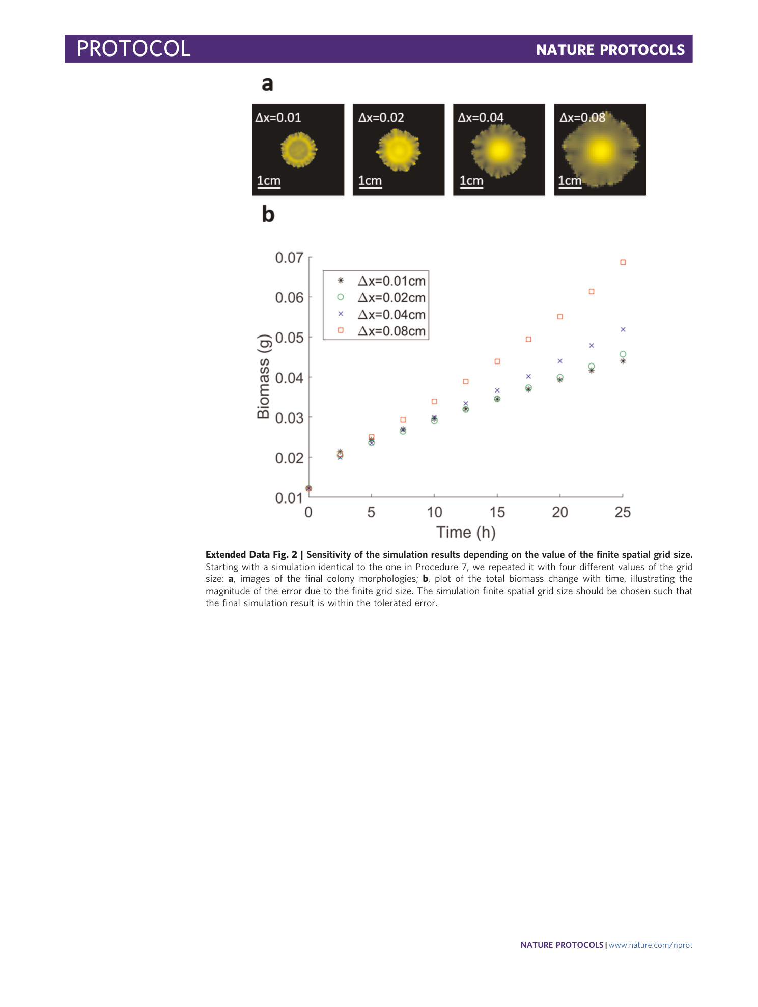
Extended Data Fig. 2 Sensitivity of the simulation results depending on the value of the finite spatial grid size.
Starting with a simulation identical to the one in Procedure 7, we repeated it with four different values of the grid size: a , images of the final colony morphologies; b , plot of the total biomass change with time, illustrating the magnitude of the error due to the finite grid size. The simulation finite spatial grid size should be chosen such that the final simulation result is within the tolerated error.
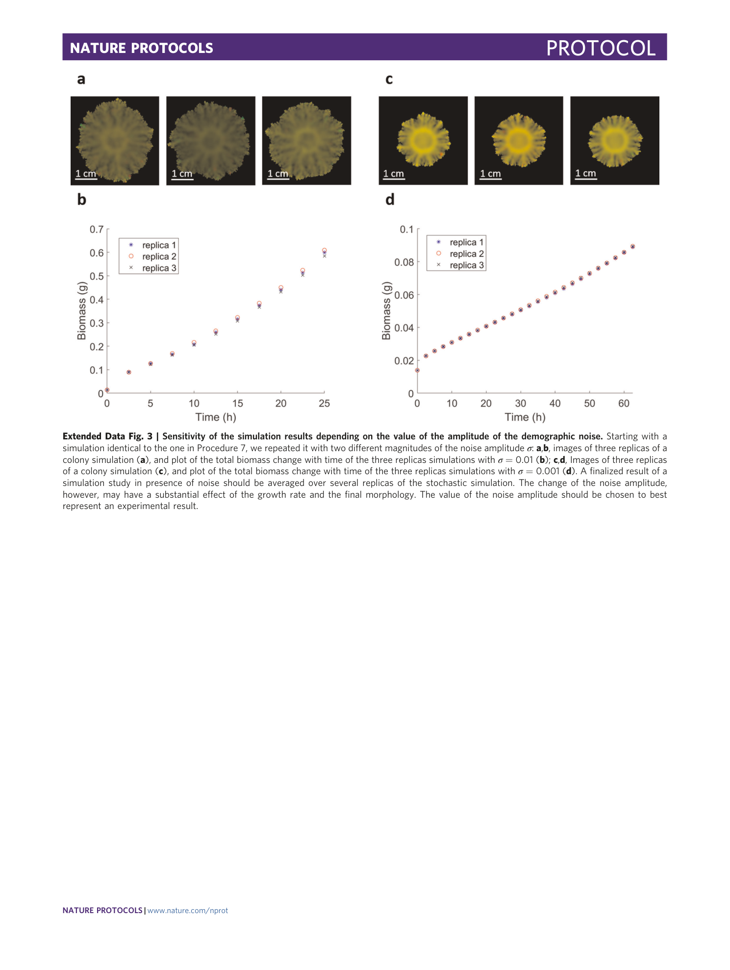
Extended Data Fig. 3 Sensitivity of the simulation results depending on the value of the amplitude of the demographic noise.
Starting with a simulation identical to the one in Procedure 7, we repeated it with two different magnitudes of the noise amplitude σ : a , b , images of three replicas of a colony simulation ( a ), and plot of the total biomass change with time of the three replicas simulations with σ = 0.01 ( b ); c , d , Images of three replicas of a colony simulation ( c ), and plot of the total biomass change with time of the three replicas simulations with σ = 0.001 ( d ). A finalized result of a simulation study in presence of noise should be averaged over several replicas of the stochastic simulation. The change of the noise amplitude, however, may have a substantial effect of the growth rate and the final morphology. The value of the noise amplitude should be chosen to best represent an experimental result.
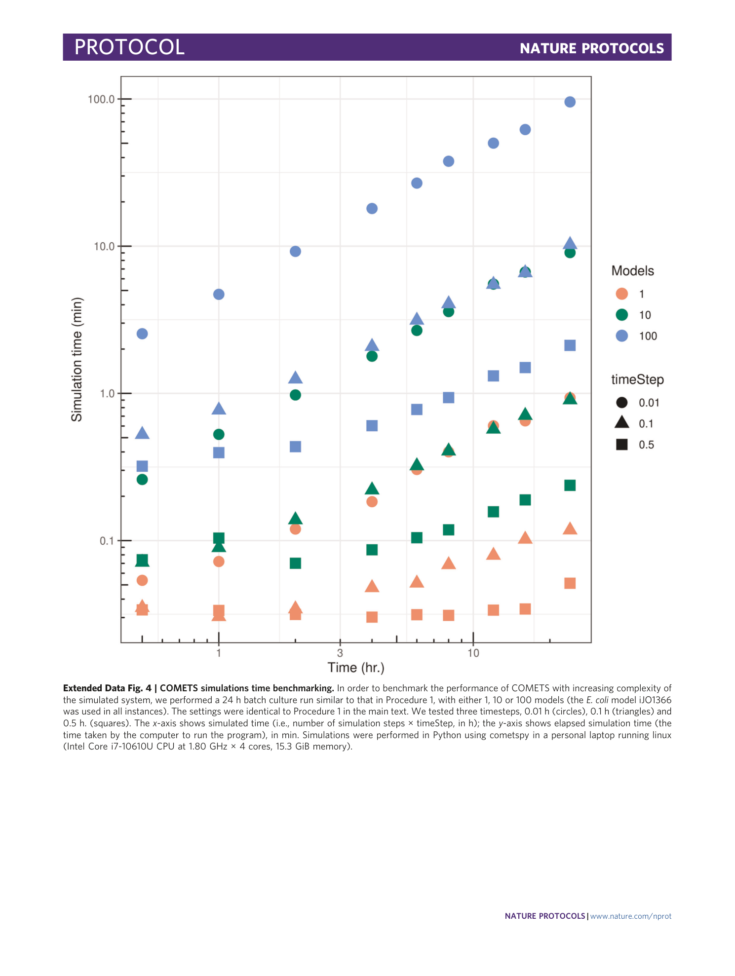
Extended Data Fig. 4 COMETS simulations time benchmarking.
In order to benchmark the performance of COMETS with increasing complexity of the simulated system, we performed a 24 h batch culture run similar to that in Procedure 1, with either 1, 10 or 100 models (the E. coli model iJO1366 was used in all instances). The settings were identical to Procedure 1 in the main text. We tested three timesteps, 0.01 h (circles), 0.1 h (triangles) and 0.5 h. (squares). The x -axis shows simulated time (i.e., number of simulation steps × timeStep, in h); the y -axis shows elapsed simulation time (the time taken by the computer to run the program), in min. Simulations were performed in Python using cometspy in a personal laptop running linux (Intel Core i7-10610U CPU at 1.80 GHz × 4 cores, 15.3 GiB memory).
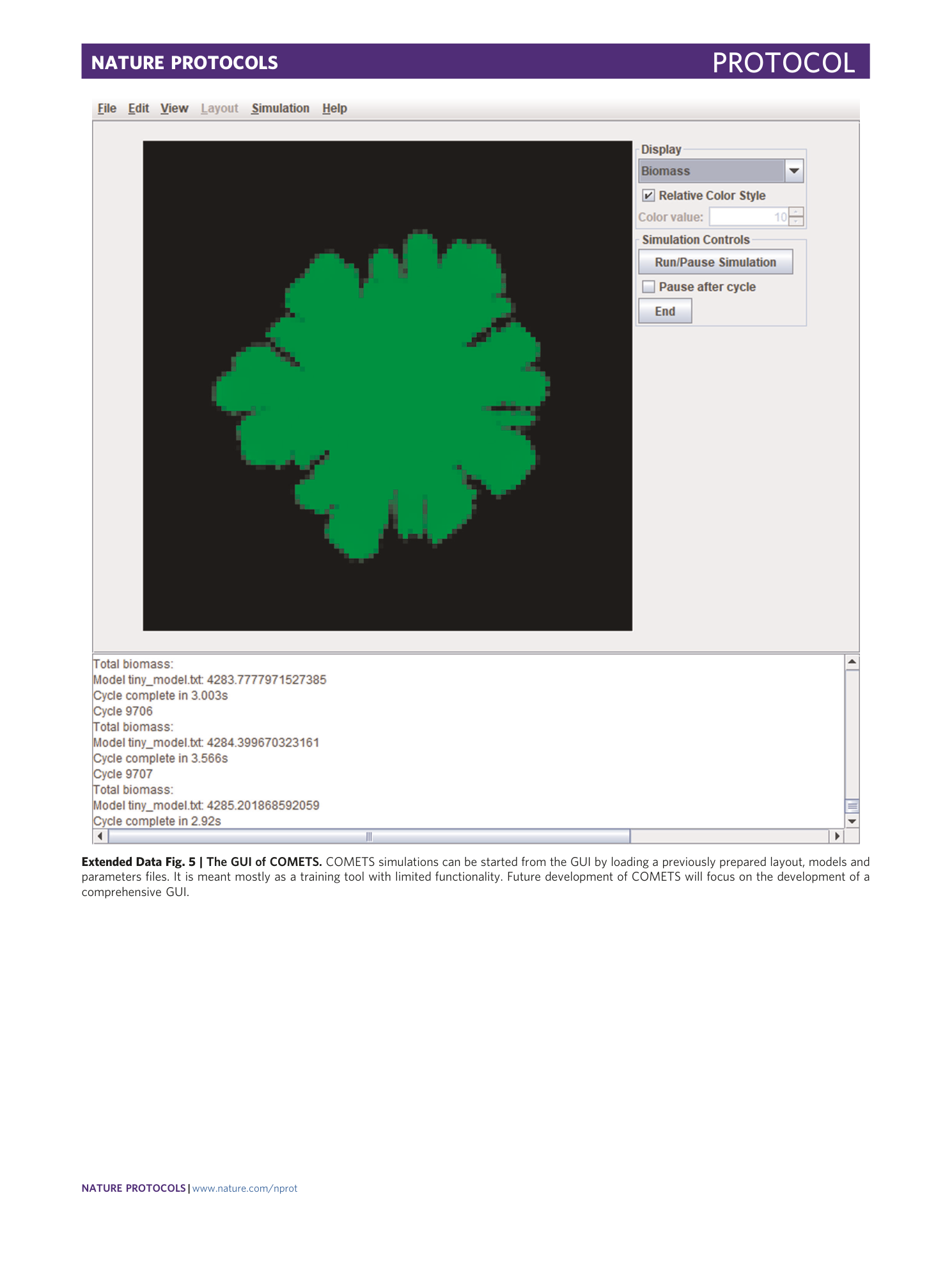
Extended Data Fig. 5 The GUI of COMETS.
COMETS simulations can be started from the GUI by loading a previously prepared layout, models and parameters files. It is meant mostly as a training tool with limited functionality. Future development of COMETS will focus on the development of a comprehensive GUI.
Supplementary information
Supplementary Information
Supplementary Discussions 1–5, Supplementary Table 1 and References.
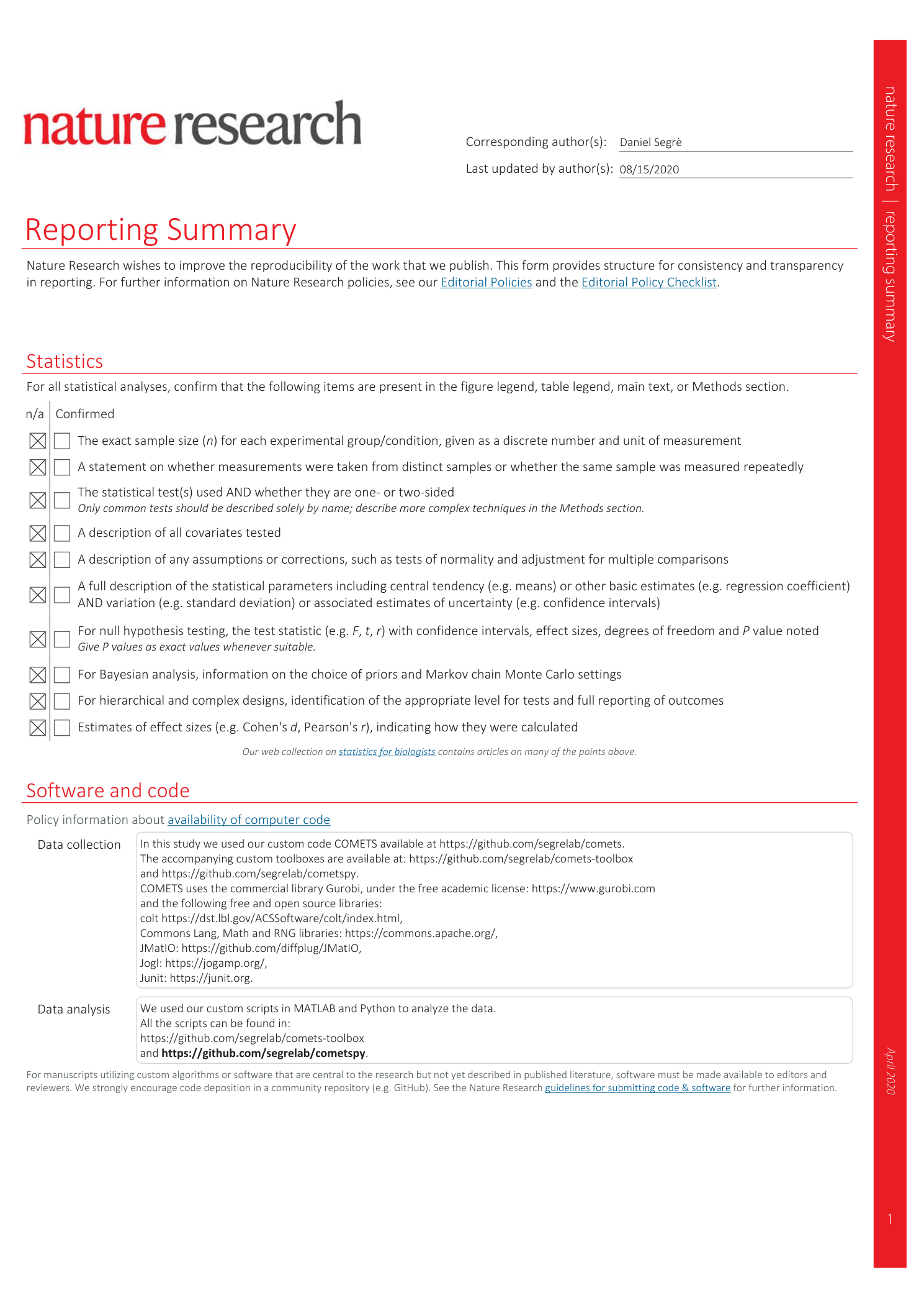
Reporting Summary
Extended Data Video 1
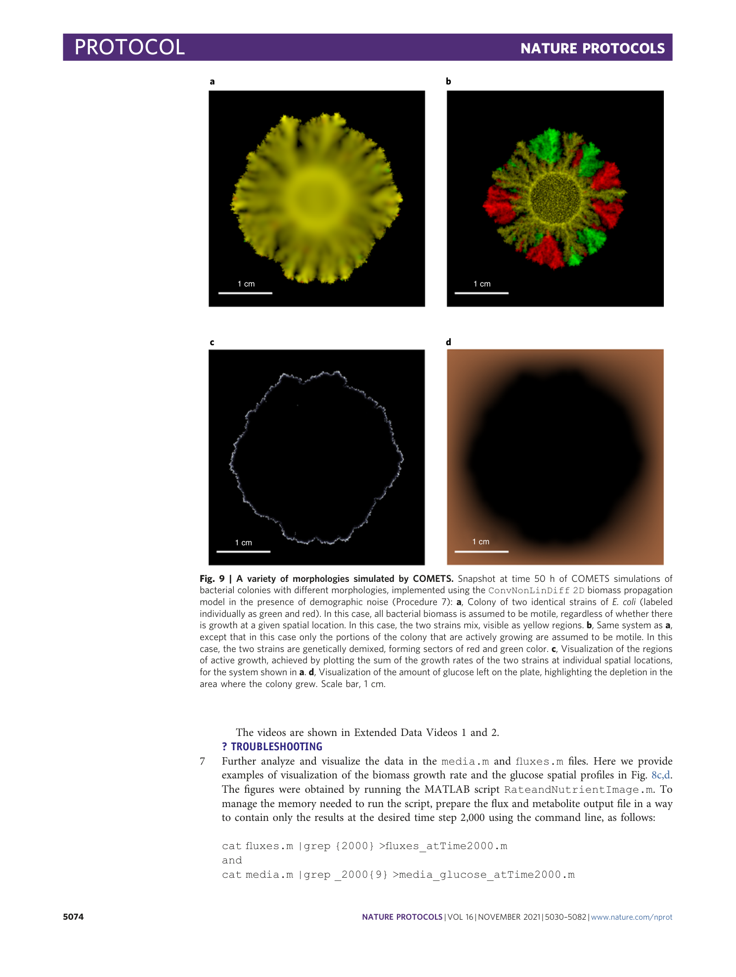
Branching colony of two identical strains of E. coli . Procedure 7, option A: growth regime without genetic demixing.
Extended Data Video 2
Branching colony of two identical strains of E. coli . Procedure 7, option B: growth regime with genetic demixing.
